It must be emphasized that these assumptions, particularly
the assumption of fixed exchange rates, present an extreme case---when
the nominal exchange rate is flexible, real exchange rate
adjustments will, as explained below, augment income adjustments in bringing
about equilibrium. A fuller analysis of the equilibrating process from
the alternative, but equivalent, aggregate demand and supply perspective
is presented in the Lessons that follow.
As in the previous Topic, the analysis here is based on the critical
equilibrium condition
We now take into account the implications of
less-than-full-employment conditions for the process by which the
desired net capital flow is brought into equality with the desired
balance on current account. To highlight essential features, we
will assume that price levels are rigid under less-than-full-employment
conditions and that the government is maintaining the nominal exchange
rate fixed. Real exchange rate movements are thus excluded as an
equilibrating mechanism.
where ΦS-I represents factors affecting the excess of savings over investment other than income and the world real interest rate, ΦBT represents the factors affecting the balance of trade other than incomes and relative prices and s , the marginal propensity to save, equals (1 − ξ) when there is continuous full employment. Since Y* and r* are determined by conditions in the in the rest of the world, DSB is determined by previous international borrowing and lending, and ΦS-I and ΦBT are constants, the only variables that can adjust to preserve the equality are the level of domestic income Y and the real exchange rate Q . Since the real exchange rate is constant as a result of the assumptions above, Y is the only variable that can adjust to maintain equilibrium.
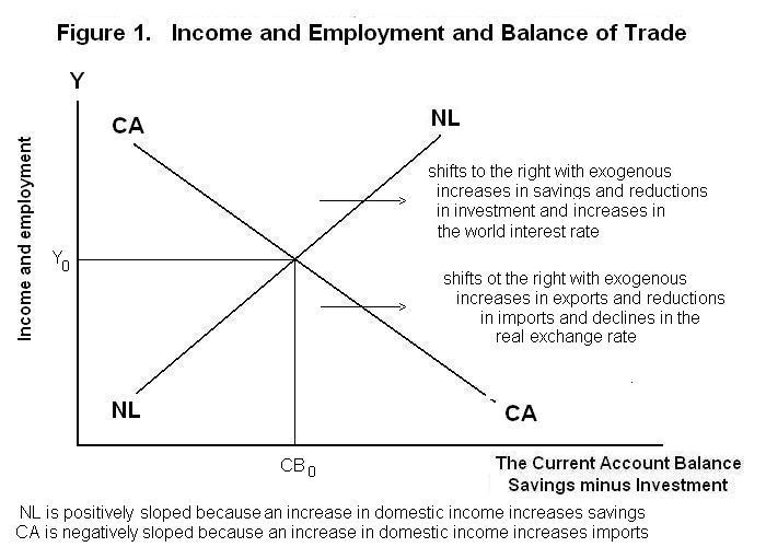
The adjustment process can be analyzed with reference to Figure 1.
The horizontal axis in measures the excess of savings over investment (or
net capital outflow) and current account balance and the vertical axis measures
the level of real income and employment. The positively sloped line NL gives
the relationship between the level of income and the excess of real savings
over real investment (net lending) as indicated by the left side of equation
above. A positive shift of savings or negative shift of investment (increase
in ( ΦS-I ) will shift the NL line to the right.
A rise in the world interest rate will reduce domestic investment, also
shifting NL to the right. NL is essentially the same as the SI
line in the figures presented in the previous Topic, except that
Y is now on the vertical axis instead of Q .
The negatively sloped CA line in Figure 1 represents the relationship between income and current account balance, given by the right side of the above equilibrium equation. As income goes up imports rise and the current account balance is reduced. A rise in the level at which the government is fixing the nominal exchange rate (increase in Π) will reduce the relative price of domestic goods in world markets, causing the current account balance to increase and shifting the CA line to the right. An increase in income abroad will increase exports and also shift CA to the right.
Equilibrium is brought about by a change in Y sufficient to bring desired net lending abroad (savings minus investment) into equality with the desired balance on current account (exports minus imports plus the debt service balance). This establishes the equilibrium level of domestic income and employment jointly with the equilibrium net capital outflow. Equilibrium occurs where the NL and CA curves cross.
Suppose that the domestic economy becomes a better place to invest than it had been previously. This will shift the NL line to the left in Figure 2.
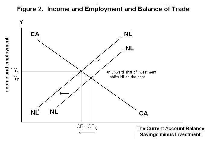
The new equilibrium will occur at a higher level of domestic real
income and a smaller net capital outflow and trade balance surplus
(or bigger net capital inflow and trade balance deficit). The
shift of investment into the domestic economy increases the aggregate
demand for domestic output. Additional output is supplied by a
reduction in the level of unemployment. The increase in output
increases imports, reducing (increasing) the current account surplus
(deficit). It also increases savings, moderating the initial increase
in net lending. Were the exchange rate allowed to change the domestic
currency would appreciate, shifting the CA curve to the left and
moderating the rise in income.
Suppose alternatively that the domestic government imposes a tariff which shifts domestic expenditure from imports to domestic goods. The effects of this are analyzed in Figure 3.
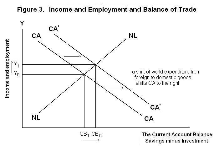
The CA curve shifts to the right. Again, the aggregate demand for
domestic output increases and is accommodated by an increase in
aggregate supply resulting from a reduction in unemployment. In
this case both output and the current account surplus (deficit)
increase (decrease). Contrary to the result in the full-employment
case, a shift of world expenditure from foreign to domestic
goods now increases the equilibrium current account balance.
Recall that under full employment conditions output could not
change and all the adjustment fell on the real exchange rate
which drove the trade balance back into equality with the unchanged
net capital inflow. If the exchange rate is allowed to change in
the present situation it would appreciate moderating the rightward
shift of the CA curve and the increase in the current account
balance---the analysis in this case is subtle, however, and a full
accounting of the consequence of exchange rate flexibility
under less-than-full-employment conditions must be postponed to
subsequent Lessons.
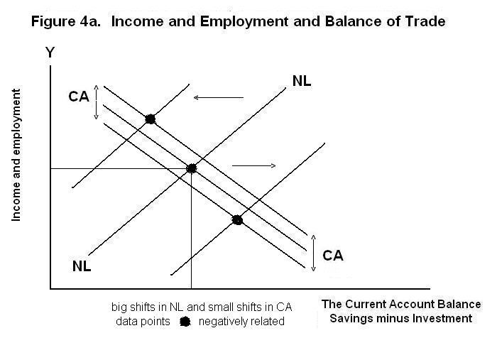
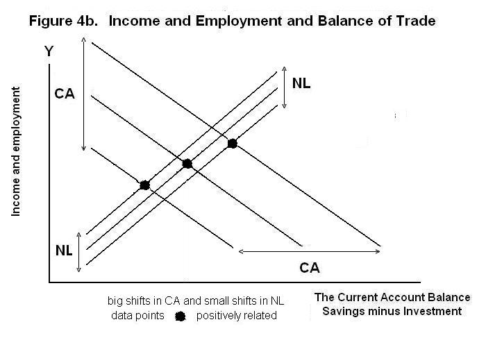
It is frequently concluded in the popular press that, since a rise in income increases imports, increases in income should always be associated with declines in the current account balance. In addition to assuming that the adjustment occurs through changes in employment and not as a result of changes in technology, this argument ignores the fact that a rise in income also increases domestic savings. It also ignores the fact that the observed movements in employment and income and the current account balance are equilibrium responses to shocks to either the current account balance or the net capital inflow or both.
If the shocks were predominantly to savings or investment we would indeed observe a negative correlation between the observed levels of income and the current account balance. If the shocks were predominantly to exports or imports, on the other hand, the observed levels of income and the current account balance would be positively correlated. This is shown in Figures 4a and 4b. Of course, if prices or the nominal exchange rate also change, all bets are off. Great care must be exercised in making from observed statistics inferences about what is actually happening.
In the less-than-full employment case, the above equilibrium
equation can be manipulated to yield an expression determining the
level of real income by bringing Y to the left side.
This is an expansion of the basic income-determination equation
Again it should be noted that nothing in the above discussion says anything about balance of payments equilibrium, which depends not on the total net capital flow or current account balance, but on the portion of the net capital flow that represents induced transactions by the government aimed at manipulating the nominal exchange rate. The factors determining balance of payments equilibrium will be analyzed in subsequent Lessons.
It is test time again. As always, think up your own answers before looking at the ones provided.
Choose Another Topic in the Lesson