From the definition of the real exchange rate
1. Q
= P / Π P*
where Q is the real exchange rate, Π is the
nominal exchange rate defined as the domestic currency price of foreign
currency, and P and P* are the domestic and
foreign price levels, we can see that the nominal and real exchange rates
will move opposite to each other when the domestic and foreign price levels
do not change. The price of foreign currency in terms of domestic currency
will rise---that is, foreign goods will become more expensive and domestic
currency will devalue in nominal terms---when the relative price of domestic
goods in terms of foreign goods falls. The real and nominal values of the
domestic currency thus move in the same direction even though the nominal
and real exchange rates, as we have defined them, move in opposite directions.
Equation 1 can be rearranged to move the nominal exchange rate to the left side
to yield
2. Π
= P / Q P*
The nominal exchange rate is the product of two terms: the
reciprocal of the real exchange rate 1/Q and the ratio of the
domestic to the foreign price level P/P*. If the real exchange
rate does not change and the domestic price level rises, Π will
rise proportionally---the external value of the domestic currency
will fall in proportion to its internal value. If Q falls, and
devalues, holding the price levels constant, the nominal exchange rate will
devalue---that is, Π will rise---in the same proportion.
Now let us suppose for the sake of argument that the full-employment real
exchange rate is constant through time and assume that the domestic authorities
expand the money supply. You should know by now that for this to happen the
nominal exchange rate must be free to rise and fall in response to market
forces. The effect of the expansion of the money supply on output and income
and/or the price level can be seen from Figure 1.
We have just finished analyzing the forces determining
movements of the real exchange rate under full-employment conditions.
Here we begin to look at forces that will affect it in
the short-run when price levels are rigid and employment can
change. We begin by looking first at the relationship between
the real and nominal exchange rates.
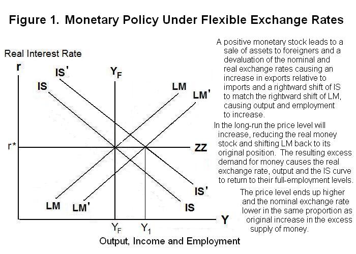
The IS curve represents the real goods market equilibrium equation
3. Y = (ΦBT + DSB − ΦS-I )/(s + m) − μ/(s + m) r + m*/(s + m) Y* − σ/(s + m) Q
where ΦS-I represents exogenous factors shifting savings relative to investment at each level of domestic income Y , s and m are the domestic marginal propensities to save and import, r* is the domestic interest rate, which is determined by conditions in the world market, Y* is foreign output and income, m* is the foreign marginal propensity to import, DSB is the debt service balance and ΦBT represents exogenous factors shifting the domestic balance of trade. And the LM curve represents the asset market equilibrium equation
4. r* = − (1/θ)( M/P − ΦM ) − τ + (ε/θ) Y
where M is the domestic nominal money stock, ΦM is a demand-for-money shift factor, and τ is the expected rate of domestic inflation. The ZZ line sets the domestic real interest rate determined by world market conditions.
You should understand by now that under flexible exchange rates equilibrium is determined by the intersection of LM and ZZ with the nominal exchange rate continually adjusting to drive IS through that LM-ZZ intersection. An increase in the money supply (or decline in the demand for money) shifts LM to the right to LM' causing domestic residents to re-balance their portfolios by purchasing assets abroad. The domestic currency devalues and Π rises, reducing the real exchange rate, shifting world demand onto domestic goods and increasing the level of output the short run when the price level is inflexible. The IS curve shifts rightward to IS' . The domestic unemployment rate falls below its normal (full-employment) level. This pressure on the labour market eventually causes nominal wages and prices to rise.
As the price level rises the real money stock declines, shifting LM back to its original position. This rise in the price level reduces the real exchange rate back to its original level, shifting IS back to its original position. When full employment is again achieved the price level and nominal exchange rate will have risen in proportion to the increase in the money supply and the levels of real output and the real exchange rate will have returned to their original levels. The monetary expansion thus has a temporary downward effect on the real exchange rate and upward effect on real income and a permanent upward effect on the nominal exchange rate and domestic price level.
The above analysis assumes that the short-run adjustment of output and employment is immediate while the adjustment in the price level takes time. In fact, however, the adjustment of output will also take time---it will take time for the devaluation of the real and nominal exchange rates to shift world demand onto domestic goods and a further period for the increased demand to increase domestic output. This has important implications for the process of exchange rate adjustment.
To see these implications, consider the stock equilibrium equation, rewritten to put the real money stock on the left side, with both sides then multiplied by P
5. M = P [ ΦM − θ (r* + τ ) + ε Y ]
An increase in M increases the left side of this equation immediately, but it will take time for something to happen to increase the right side. During this time interval domestic residents will have excess money holdings and will be trying to exchange them for assets on the international market. Although the adjustment of output will take time, the exchange of money for assets and the associated pressure on the exchange rate will occur almost immediately. The upward movement of the nominal exchange rate, and corresponding downward movement of the real exchange rate, will explode unless something happens to bring the two sides of the asset equilibrium equation into equality. This prompts us to delve more deeply into the question of how we measure the price level.
We have written the asset equilibrium equation using the price level of domestic output as our price variable. In fact, however, we should measure the real money stock using the price index of goods absorbed or bought by domestic residents. These goods have traded and non-traded components. The prices of the non-traded and traded components of output in domestic currency can be denoted as PN and PT respectively. The price level that should be used in Equation 4 is thus
6. P' = w PN + (1 - w) PT = w PN + (1 - w) Π PT*
where w is the share of the non-traded components in total domestic absorption and (1 - w) is the share of traded components.
The asset or stock equilibrium equation must now be written
7. M = P' [ ΦM − θ (r* + τ ) + ε Y ] = [ w PN + (1 - w) Π PT*] [ ΦM − θ (r* + τ ) + ε Y ]
An increase in the nominal exchange rate will directly raise the properly defined domestic price level in Equation 7 in the proportion (1 - w) . The rise in P' will be less than the rise in Π because (1 - w) < 1 . Since P' must rise in proportion to the rise in M to reestablish asset equilibrium when nothing else has yet had time to adjust, a rise in Π in excess of the rise in M and in excess of the long-run equilibrium rise in Π must occur in the short-run. Exchange rate overshooting takes place---the exchange rate overshoots its new long-run equilibrium in the short-run during process of getting to that long-run equilibrium.
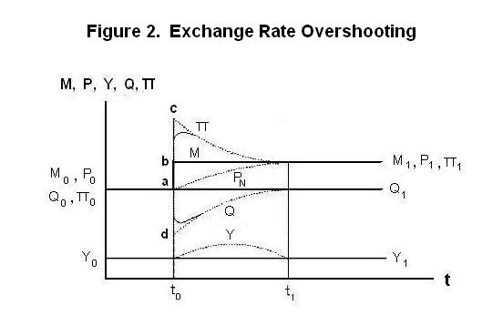
This is illustrated in Figure 2. When everything including the price level adjusts immediately, M , P and Π will all shift up by the amount a b at time t0 and remain at their new levels indefinitely. And Q and Y will remain constant. When income and prices cannot adjust immediately, Π will jump all the way up to c and then gradually fall back to its long-run equilibrium level. The real exchange rate Q will jump down to d and then gradually rise back up to its original level. The price level of the non-traded component of output PN will rise gradually, as shown by the dotted line, to its long-run equilibrium level which will be the same as the long-run equilibrium levels of PT and Π PT*. And Y will rise temporarily relative to its long-run level while the prices are adjusting. When time t1 is reached, everything will be back in long-run equilibrium.
Economists can say with certainty that the adjustment will be of the sort described above and portrayed in Figure 2, but they cannot predict with any precision in real-world cases the exact magnitude of the overshooting or length of time required for long-run equilibrium to be achieved. If people know that the government is increasing M they will adjust wages and prices immediately unless they are locked into long-term contracts---nobody would willingly take less than the optimal wage or price. Then t0 and t1 will occur almost simultaneously. When it takes a long time for people to learn that M has changed or when wages and prices are temporarily fixed by contract, t0 and t1 will be far apart. The adjustment lag is likely to be different in each real-world situation depending on the circumstances.
There is a mechanism that will moderate overshooting exchange rate movements in certain circumstances. You will recall from studying the computer-assisted learning module entitled The Foreign Exchange Market that the domestic real interest rate is related to the foreign real interest rate according to the equation
8. r = r* + ρ − EQ
where ρ is the risk premium on domestic assets and EQ is the expected rate of increase in the real exchange rate. An expected increase in the real exchange rate will increase the expected future value of---that is, yield a capital gain on---domestic capital goods, making asset holders willing to hold domestic capital at a lower market real interest rate.
An overshooting movement of the nominal and real exchange rates will by definition be corrected by a movement in the opposite direction. When there is known to be an overshooting devaluation, the expectation will be that Q will rise in the future, so that EQ then become positive and the domestic interest rate will fall, making people willing to hold some of the excess money holdings that led to the devaluation. This will moderate the degree of overshooting of the nominal and real exchange rates, rounding off the peaks at c and d in Figure 2.
Interest rate adjustments that moderate the degree of overshooting will occur only if people are able to discern that overshooting is in fact taking place. If real the exchange rate is perceived to be a random walk, which scientific evidence suggests best describes its short-run movements, EQ will be unaffected by the change in Q and no moderation of the overshooting will occur---the best forecast of tomorrow's exchange rate turns out to be today's. But one cannot rule out the possibility that certain shocks to the exchange rate could be viewed by a significant segment of the market to be overshooting shocks, even though in general the real exchange rate exhibits close to random walk behavior.
Essentially the same exchange rate overshooting process will occur when there are shocks to the demand for money. In this case the right side of Equation 7 will shift with the left side remaining unchanged. The immediate adjustment of the exchange rate required to bring the two sides into equality will overshoot its ultimate long-run equilibrium level.
The government could prevent overshooting adjustments of the exchange rate resulting from demand for money shocks by varying the supply of money to offset them, keeping the two sides of Equation 7 equal. To do this, of course, it would have to know when the demand for money is shifting and by how much.
Time for a test. Be sure to think up your own answers before looking at the ones provided.
Question 1
Question 2
Question 3
Choose Another Topic in the Lesson.