It is now time to begin a more rigorous analysis of the behaviour of the firm
than was presented in the two earlier lessons dealing with microeconomics. We
start with a situation where there are many firms producing a homogeneous
product so that perfect competition prevails. This analysis is conducted with
reference to Figure 1 below, which focuses on a typical firm.
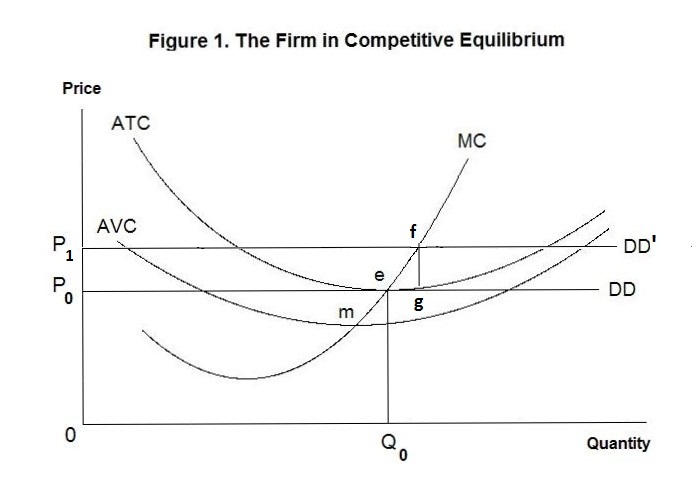
The curve AVC gives the firm's average variable cost curve. Total variable costs increase at an increasing rate as output increases. Average variable costs---that is, total variable costs divided by the quantity of output produced---falls as output increases when output is low and rises as output increases when output becomes large. The minimum point on the average variable cost curve is at point m. The firm also has fixed costs, which are independent of the level of output---average fixed costs thus decline continuously as output increases. When we add average fixed costs to average variable costs we obtain the average total cost curve, denoted as ATC. Since average fixed costs become smaller as output increases, so does the vertical distance between the AVC and ATC curves---the minimum point on the average total cost curve, at point e, thus occurs at a higher level of output than the minimum point on the average variable cost curve. The marginal cost curve, denoted as MC, gives the change in total cost associated with a one unit change in output. It is equal to average variable cost when average variable cost is at its minimum---at that point a small change in output increases total variable costs in the same proportion as that increase in output, thereby having no effect on average variable costs. And, for the same reason, marginal cost is equal to average total cost when average total cost is at its minimum. Thus, the marginal cost curve rises continuously as output increases beyond some level below that where average variable cost is minimum.
When there is perfect competition and the output good produced be each firm is identical to that produced by all other firms, the individual firm's demand curve is a horizontal straight line, denoted in Figure 1 by DD. Each firm will increase its output whenever the increase in its total revenue from producing an additional unit exceeds the increase in its total cost---that is, whenever marginal revenue exceeds marginal cost. Since the price of the firm's output is unaffected by the amount it produces, its marginal revenue is everywhere the same, and equal to P0 where the DD line crosses the vertical axis. Where all firms have identical total cost curves they will all produce at the minimum points on those curves where marginal cost equals price.
Of course, in the real world some firms will be better managed than others with the result that their total costs are lower. This means that their minimum average total cost will be less than the market price. They will produce where marginal cost equals price and earn a slight profit. But we can think of this profit as a return on managerial skill which could be earned in some other industry as well as in this one. Accordingly we can include that profit as a cost of being in this industry rather than elsewhere and simply add it to the firm's total cost. The minimum point of this new total cost curve will then be equal to price and Figure 1 will continue to present a correct picture.
Now let us relax the assumption that the output produced by all firms consists of quantities of an identical good. This assumption is ridiculous for all but a very few industries---for example, coke and pepsi are not viewed the same by soft-drink consumers, and the quality and type of service provided by local convenience stores differs somewhat. By raising its price, therefore, the firm will not suffer a complete loss of demand for its output. It's demand curve will then have a slightly negative slope as indicated by the curve DD in Figure 2 below. Given this negative slope, the firm's marginal revenue curve, denoted as MR, will be below the demand curve at every output in excess of one unit. The firm's output will be at point Q0 where marginal revenue equals marginal cost, below the output level where average total cost is at its minimum.
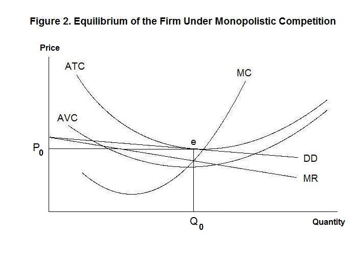
But why, in the Figure above, is the average total cost curve tangent to the demand curve? Why can't the firm, since it has some control over the price at which it sells its output, earn some monopoly profit? After all, it is the only producer in the economy of the specific product it is selling, given that its product is slightly different from those produced by all other firms. Here it should be recalled that there are many firms in the industry producing very similar products. If those firms took advantage of product differentiation to raise their output price sufficiently to earn revenue in excess of their costs, new firms would enter the industry to share in these profits---this will reduce product prices, shifting all firms' demand curves downward. Equilibrium will occur when there are no potential benefits to new entrants at which point the demand curves facing all firms in the industry will be tangent to their total cost curves. Of course, as in the case of perfect competition, some firms may be more efficient than others but, again, such excess profits can be treated as costs that represent wages for the managerial skills of these firms' owners.
Finally, we examine the equilibrium conditions for a monopolistic firm---one that is the only producer of a product for which there are poor substitutes. The firm's equilibrium is presented in Figure 3 below.
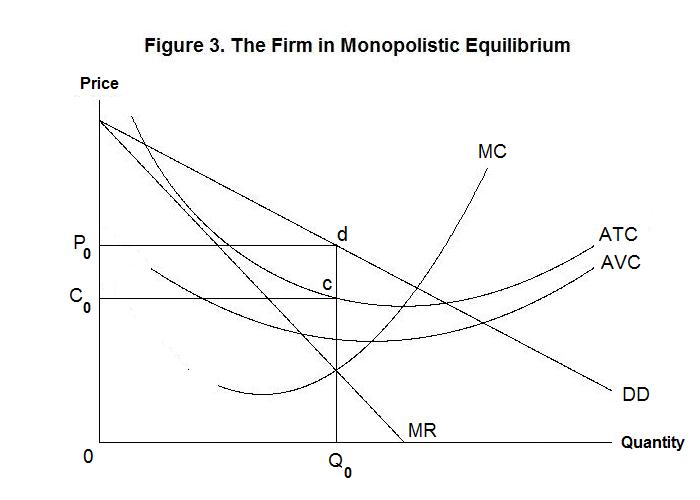
The firm produces where its marginal revenue equals its marginal cost, at output Q0. It charges a price P0 and its average total cost is C0, yielding a monopoly profit equal to the rectangle P0 d c C0.
It is test time. As usual, think up your own answers before looking at the ones provided.
Choose Another Topic in the Lesson