It is obvious that an unemployed worker willing to work for
next to zero pay would find employment almost immediately. At
higher reservation wage rates, however, the process of matching
worker to job takes time. Workers can be thought of as setting
reservation wage rates, adjusted to compensate for expected job
satisfaction, and then presenting themselves sequentially to firm
after firm until they are hired. The waiting time until employment
is found is thus a random variable that depends on the luck of the
draw as the worker goes from firm to firm. There is a small probability
of being hired very quickly, a large probability of having to wait for
a substantial time and a small probability of having to wait a long time.
Moreover, we would expect the average, mean, or expected waiting time to
increase as the reservation wage increases.
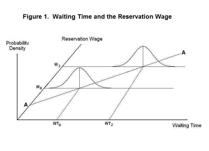
The situation can be analyzed in Figure 1. The line AA gives
the relationship between mean waiting time and the reservation wage.
Centered on the mean waiting time associated with each reservation
wage is a probability distribution of actual waiting times. Two
of the infinitely many such probability distributions are drawn,
associated respectively with the mean waiting
times WT0 and WT2.
Probability is measured on the vertical axis. All probability
distributions are scaled so that the areas under them equal unity
in recognition of the fact that the probability that some waiting
time will occur is unity. Half of the area lies to the left of the
mean waiting time and half to the right in recognition of the fact
that there is a 50 percent chance that waiting time will be above
the mean and a 50 percent chance that it will be below the mean.
We now break with the neo-classical tradition by assuming
that workers and jobs are not homogeneous. Each worker differs in
important respects from his/her peers---in intelligence, attitude,
trustworthiness, judgment, embodied human capital and, hence,
general competence. Although identical jobs do exist, many jobs
require slightly different skill attributes and yield somewhat
different satisfaction to those performing them. The worker is
thus assumed to be a monopolistic competitor in the job market.
Leaving the explanation of layoffs to the next Topic, we here
address the issue of the length of time it takes an unemployed
worker to find a job.
The probability distribution associated with the mean waiting time WT0 is blown up in Figure 2. The unit area under the curve is divided into regions. The probability that the waiting time will be between the boundaries of each region along the horizontal axis is equal to the area of that region as a fraction of unity. For example, the probability that the time it takes to find a job will be between WT0 and WT1 is .20 + .20 = .40, or 40 percent. And the probability that it will take longer than WT1 to find a job is .05 + .05 = .10, or 10 percent. Similarly, the probability that the waiting time will be less than or equal to W3 is .05, or 5 percent.
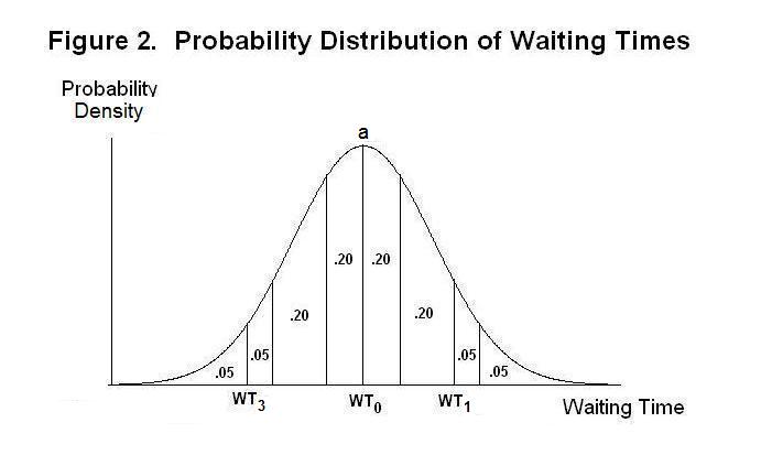
The probability that it will take in the neighborhood of WT0 to find a job is given by the length of a very thin vertical strip running between the horizontal axis at WT0 and point a . This says that the most likely waiting time is WT0. Waiting times greater or less than WT0 are less likely to occur as can be seen from the fact that the curve, which is called the Probability Density Function, is closer to the horizontal axis at all points to the left and right of WT0. The area under the curve to the left of a given waiting time gives the cumulative probability---that is, the probability that the waiting time will be less than or equal to that amount. The probability that waiting time will be less than or equal to WT0, for example, is 0.5 .
Now suppose that the central bank reduces the money supply, or that the demand for money increases, so that the new full-employment equilibrium nominal wage rate becomes W1 in Figure 3. A reduction in the price level and all nominal wage rates proportional to the reduction in the money supply or increase in the demand for money must ultimately occur, with the real wage rate remaining constant. Suppose also that everyone in the economy knows what has happened. Workers' new probability distribution of waiting times at nominal wage rate W1 is given by the probability density function centered at point b.
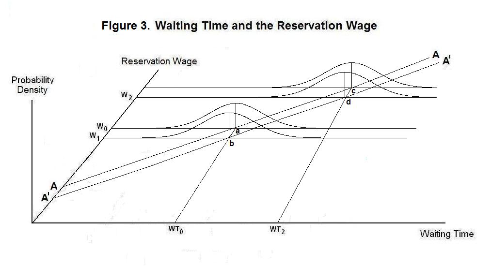
Since workers know what is happening, it is in their interest to reduce their reservation wage to W1 and, given the proportional fall in the price level, their real wage rate will remain constant at that point. Had they wanted to choose a different equilibrium waiting time, they would have done so before the nominal money shock occurred. Average waiting time will remain at WT0 and unemployment will remain at its natural or full-employment level. This is the case of wage and price flexibility and full employment.
Now suppose that workers do not know that monetary conditions have tightened and the new full-employment equilibrium wage rate has fallen to W1. In the absence of any knowledge that things have changed, they maintain their reservation wage rate at W0. At that reservation wage rate, the probability distribution of waiting times has shifted to the right to the one centered on point b in Figure 4. As a result, the average waiting time of workers before finding jobs will rise to WT1. Unemployment will thus rise above its natural rate.
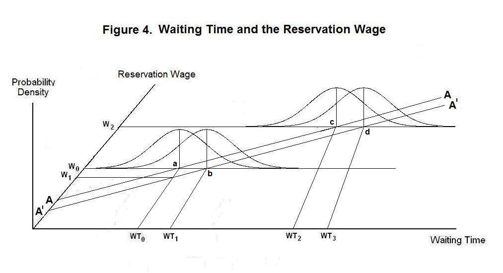
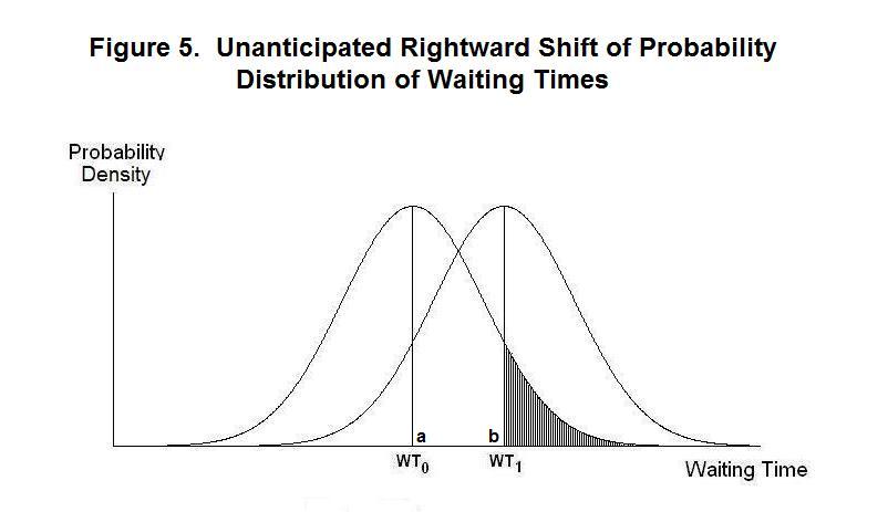
As this happens workers will observe that it is taking them longer to find jobs than they expected. But until the problem has persisted for some time, they will have no way of knowing that the higher waiting time is not a low-probability event that, as shown by the shaded area in Figure 5, would have an approximate 10 percent chance of occurring at unchanged aggregate demand and mean waiting time. Only after higher waiting times have persisted for some time will workers realize that the decline in aggregate demand has occurred. Once they realize this, they will reduce their reservation wage to W1 and average waiting time and the unemployment rate will return to their equilibrium levels.
Unemployment---that is, a rise of the unemployment rate above its natural level---thus occurs as a result of shifts in aggregate demand that take workers by surprise. Once they realize the extent of any aggregate demand shift they will adjust nominal, and hence, real wages to levels consistent with normal waiting times to find jobs. And the unemployment rate will then return to its natural level.
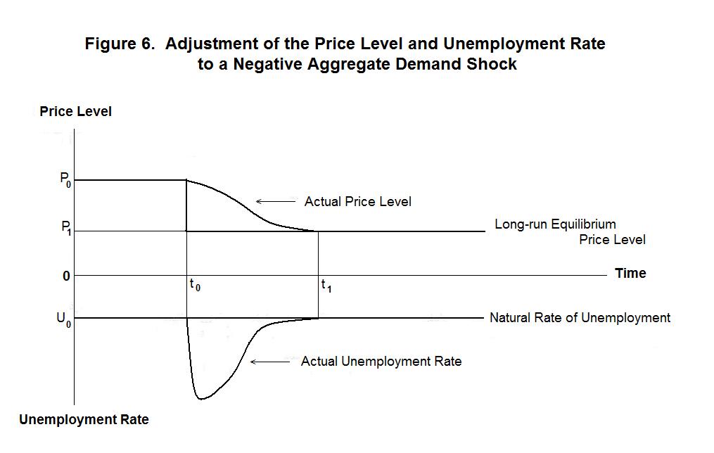
The time-path of adjustment of the unemployment rate and price level to a decline in nominal aggregate demand is illustrated in Figure 6. The long-run equilibrium price level, given by the upper thick line, jumps down at time t0 when aggregate demand declines. The unemployment rate, given by the distance of the lower thick line below the zero line, increases sharply as workers, being unaware that aggregate demand has shifted, are fooled into over-pricing themselves. The actual price level falls slowly as workers realize what has happened and cut their reservation wages, and firms pass these lower wages on to consumers in lower prices. By time t1 wages and prices have fallen to their new long-run equilibrium levels and unemployment has returned to its natural rate.
Similarly, unexpected positive shocks to aggregate demand will cause the unemployment rate to fall below its natural level. Workers, failing to realize that nominal aggregate demand has increased, will maintain their reservation wage rates at levels that are too low and end up finding jobs quicker than they expected. Only after some time has elapsed will they learn that they are underpricing themselves and raise nominal wages to the equilibrium level, at which point the unemployment rate will return to its natural level.
The above analysis provides a very good explanation of observed fluctuations in the unemployment rate as the economy goes through periods of boom and bust. But it leaves important details unaddressed. It does not explain why firms actually lay off workers. Nor does it explain why workers quit their jobs more frequently in boom periods when wages are rising and desperately hang onto jobs in recessions when wages are declining. To address these and some other issues we need a contract theory of wage setting---the subject of the next Topic.
The question that naturally arises is: What determines the natural rate of unemployment? One obvious factor is the degree of labour turnover in the economy. A faster rate of technological change, for example, would require more frequent displacement of workers from old-technology jobs and their movement to jobs using new technology. This would mean that more workers will be in the process of finding new jobs at any point in time and that the natural rate of unemployment will be higher. A second factor affecting the natural rate of unemployment is the government's policy with respect to unemployment insurance. If there is generous public provision of unemployment insurance it will be less costly for workers to be unemployed and they will have less incentive to find jobs quickly. They will be inclined to set their reservation wages higher and expect to take longer to find jobs. The opportunity cost of working instead of taking leisure has increased, and workers can be expected to spend longer times between jobs. By raising their reservation wage rates, they not only increase the time it takes to find a job, raising leisure, but also increase the wage they will receive when a job is found.
It is time again for a test. Be sure to think up your own answers before looking at the ones provided.
Question 1
Question 2
Question 3
Choose Another Topic in the Lesson