1. Q
= P / Π P*
where P is the domestic price level, P* is the price
level in the rest of the world and Π is the nominal exchange
rate defined as the domestic currency price of foreign currency. As noted many
times previously, the real exchange rate can be thought of as the price of
domestic output in terms of foreign output.
You will also recall that under full-employment conditions the real exchange
rate must continually adjust to maintain equality between the desired current
account balance and the desired net capital outflow---this follows from the
condition of flow or commodity market equilibrium developed in previous
computer-assisted learning modules, which can be expressed in one of its forms
as
2. ΦS-I
+ s Y + μ r* = ΦBT
− m Y + m* Y* − σ Q
+ DSB
where ΦS-I = − (a
+ δ) represents exogenous factors shifting consumption and
investment respectively that thereby affect the excess of savings over
investment at each level of domestic income Y , s and
m are the domestic marginal propensities to save and import,
r* is the domestic interest rate, which is determined in the world
market, Y* is foreign output and income, m* is the
foreign marginal propensity to import, DSB is the debt service
balance and ΦBT represents exogenous factors
shifting the domestic balance of trade. The desired net capital outflow
appears on the left side of the equality and the current account balance on the
right side. To maintain goods market equilibrium under full-employment
conditions the real exchange rate Q must adjust through changes in
either the nominal exchange rate or the price level to ensure equality of the
left and right sides.
This real goods market flow equilibrium equation can be manipulated to yield an
expression determining the real exchange rate by bringing Q to the
left side.
3. Q = −
(1 / σ) [ ΦS-I + s Y + μ
r* ] + (1 / σ) [ ΦBT − m
Y + m* Y* + DSB ]
The real exchange rate Q is determined by movements in domestic
and foreign incomes, the world-market-determined domestic real
interest rate r* and the exogenous shift
variables ΦS-I and ΦBT .
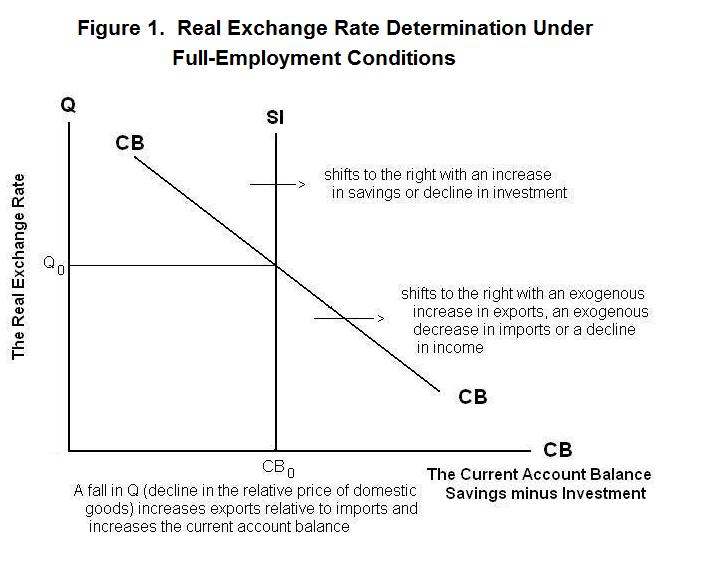
The process by which equilibrium is achieved under full-employment conditions
can be seen with reference to Figure 1. The vertical line SI gives the
desired net capital inflow---it shifts to the right with an exogenous increase
in savings or decrease in investment. It is vertical because the net capital
flow is not affected by changes in the real exchange rate when domestic and
foreign incomes and the real interest rate remain the same. The line CB gives
the relationship between the real exchange rate and the current account
balance---a fall in the real exchange rate causes the current account balance
surplus, measured along the horizontal axis, to increase. An exogenous
increase in exports or reduction in imports shifts this curve to the right.
Equilibrium occurs where the desired net capital outflow equals the current
account balance.
Our next task is analyze the determinants of the real
exchange rate more closely. You will recall that the real
exchange rate Q is equal to
Exogenous shocks to the net capital flow represented by changes in ΦS-I shift the SI line and cause the real exchange rate to adjust to create an equivalent change in the current account balance. Exogenous shocks to exports and imports represented by changes in ΦBT shift the CB curve. Since the vertical SI line remains in position, the real exchange rate has to adjust to keep the current account balance equal to the unchanged net capital flow. The current account balance is thus unaffected.
The path of the real exchange rate through time as saving, investment and technological change occur and the full-employment levels of domestic and foreign output and the real interest rate evolve will thus depend on how ΦS-I and ΦBT change through time.
A less formal way of thinking of this process is to build on the fact that the real exchange rate is the relative price of domestic output in terms of foreign output. This relative price will be determined, like all relative prices, by supply and demand. An increase in the world demand for domestic relative to foreign output will cause the price of domestic output in terms of foreign output---the real exchange rate---to rise. An increase in the supply of domestic relative to foreign output will cause the real exchange rate to fall. So the time path of the full-employment real exchange rate will depend on the evolution of the demand and supply of domestic relative to foreign output through time. Government policy will affect this process to the extent that it causes domestic and rest-of-world demand to shift between foreign and domestic goods.
Technological change and the growth of the capital stocks in the domestic and foreign economies will determine how the relative supplies of the two outputs evolve through time. These same factors, because they determine domestic and foreign incomes, will also determine the evolution of the demands for domestic and foreign output through time. Because a crucial element here is technological change, which is impossible to quantify, the exact confluence of forces that determine the movements of the full-employment real exchange rate in practical real-world cases remains a mystery, given the present state of economic science.
Economists can speculate, sometimes correctly, that a shock to oil prices or a change in government policy that affected domestic savings or investment or shifted world demand onto domestic goods caused a particular observed movement in a country's real exchange rate. But coherent detailed explanations of real exchange rate movements over extended time periods are difficult to come by.
Forecasting movements in the real exchange rate is even more difficult, for two reasons: First, it is difficult to establish the quantitative relationship between technological and policy developments and the real exchange rate. Second, even if we knew these relationships precisely, we would have to correctly forecast the future path of technological change and the various political forces affecting government policy. It is thus not surprising that economists have found that the naive forecast that the real exchange rate will remain the same between this period and next, while nearly always wrong, is virtually impossible to improve upon. More elaborate forecasts typically lead to larger prediction errors.
Economists have found that actual real exchange rate movements can be roughly described by equations of the sort
4. qt = qt-1 + εt
where q is the logarithm of the real exchange rate and εt is a random or stochastic variable that is equally likely to be positive or negative but will average out to zero. This equation can be rearranged as
5. qt − qt-1 = εt
which says that the real exchange rate will change from period to period by an amount which is equally likely to be positive as negative. In this case the exchange rate is said to follow a random walk.
This random walk process must be distinguished from another process described by the equation
6. qt = qm + εt
where q deviates from some average level qm in each period by an amount εt ---every period q reverts back to its mean or average value before being perturbed again by the shock εt . This contrasts with the previous case where the real exchange rate is perturbed each period from last period's level rather than from some constant average level. In equation 6, the exchange rate deviates randomly from its average level while in equations 4 and 5 it wanders randomly with no fixed anchor.
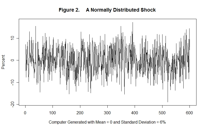
Figure 2 gives an example of a mean centered process of the sort described by equation 6. Figure 3 gives three examples of random walk processes described by equations 4 and 5. Only one example of a mean centered process is given because all such processes look pretty much the same. As can be seen from Figure 3, however, random walk processes can generate a wide variety of different paths.
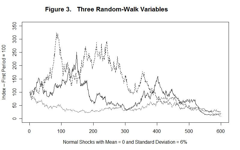
All of the examples in Figures 2 and 3 are derived from the same statistical process generating estimates of εt . Three sequences of 600 estimates of εt were generated. The first appears in Figure 2 and it and the remaining two sequences were used to generate the series in Figure 3.
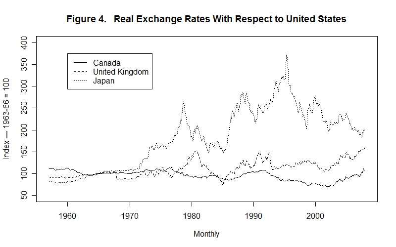
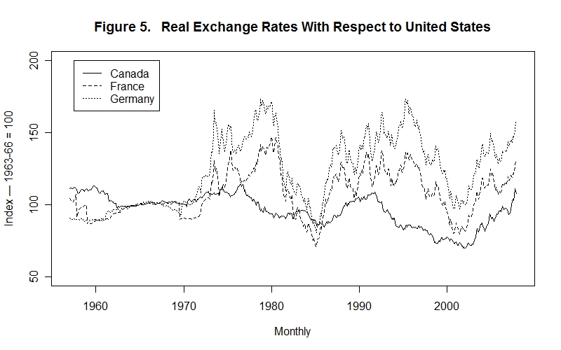
These artificially generated series can be contrasted with the actual real exchange rate movements over the past 50 years for Canada, the United Kingdom and Japan with respect to the United States, shown in Figure 4, and for Canada, France and Germany with respect to the United States, shown in Figure 5. The similarities in the type of variability of the series in Figure 3 with those in Figures 4 and 5 are obvious. Actually, it turns out that actual real-world real exchange rate series are usually not true random walks---there is typically some tendency for positive shocks to get smaller when the real exchange rate is above the mean and negative shocks to get smaller when it is below the mean. But these tendencies to mean-revert over the long run are not apparent to the naked eye.
This random-walk character of real exchange rate movements is consistent with the finding that usually the best predictor of tomorrow's exchange rate is today's. Real exchange rates exhibit this random-walk behavior because the factors determining them are equally likely to have positive as negative effects in any given period. This does not mean, of course, that real exchange rates are randomly determined---it means simply that they appear to us as randomly determined. The variable εt is a measure of our ignorance as to what is really going on.
Time for a test. As always, think up your own answers before looking at the ones provided.
Question 1
Question 2
Question 3
Choose Another Topic in the Lesson.