a) Equality of the flow of domestic output of goods
and services produced with the desired absorption of domestic goods
and services by domestic and foreign residents for consumption and
investment purposes.
b) Equality of the existing stocks of domestically
employed assets held by domestic residents and foreigners with
the quantities of those assets they desire to hold.
The capital stock employed in the economy must be willingly owned by
domestic and foreign residents and the flow of output generated by that
capital stock must be willingly bought by domestic and foreign residents
with an expenditure equal to the cost of producing them.
The first component of this overall equilibrium can be termed
flow or goods market equilibrium, and the second, stock or asset
market equilibrium.
This topic deals entirely with goods market equilibrium and
is in large part a review of material you should have already worked
through in the module entitled The Balance of Payments and
the Exchange Rate. The derivations there are reproduced here from
a slightly different perspective and then presented graphically in
an alternative form.
The purchases of domestic output by the domestic and foreign private sectors
and government consist of domestic consumption goods, domestic investment
goods and goods exported to foreign residents. Thus,
1. X = C'
+ Ig' + E'
where C' is real domestic consumption goods and services,
Ig' is real domestic investment goods and services and
E' is domestically produced goods and services
purchased by foreign residents.
The domestic private and government sectors also import goods and
services for consumption and investment and re-export. Denoting
foreign variables by placing a ˆ on top of them, total imports
can be expressed as
2.
Ê = ÊC
+ ÊI + ÊE
where Ê is total domestic imports (= foreign exports)
and the three terms to the right of the equal sign are, respectively,
imports of consumption, investment, and re-exported goods and
services.
We now add the right-hand-side of Equation 2 to and subtract the
left-hand-side of that equation from the right-hand-side of
Equation 1 and consolidate the terms to obtain
3. X = C
+ Ig + E − Ê
where C is real domestic consumption of domestically produced
and imported goods and services, Ig is gross real domestic
investment inclusive of imported goods and services and E is
domestic exports inclusive of imported goods that are later re-exported.
Now we can subtract depreciation of domestic capital, denoted by D ,
from both sides of Equation 3 to obtain
4. Ÿ
= X − D = C
+ I + E − Ê
= C + I + BT
where Ÿ is total income generated in the domestic economy,
BT ( = E − Ê )
is the balance of trade in goods and services, excluding the services of capital,
and I ( = Ig − D )
is net investment---the net additions to the stock of domestically employed
capital. We have consolidated private and government transactions so
that consumption, investment, and net exports are the combined private and
public expenditures on these goods and services.
The total income of domestic residents is equal to income produced in the
domestic economy minus interest and dividends paid to foreign residents plus
interest and dividends earned abroad by domestic residents---that is,
Y = Ÿ + DSB
where DSB is the debt service balance. Equation 4 can then be
modified to yield
5. Y
= C + I + BT + DSB
where BT + DSB is the domestic current
account balance.
Equation 4 can be interpreted as an equilibrium condition.
If C , I , and BT are interpreted as
desired magnitudes, and (Y − DSB) is the level of
output, net of depreciation, that firms actually produce, then economic
variables must adjust to ensure that equilibrium occurs---that desired
expenditure on domestic output equals the value of output produced.
Alternatively, Equation 4 can be treated as an aggregate demand equation
and expanded by substituting in the relationships determining desired
consumption, investment and the balance of trade. You should already
understand that real consumption is determined by
6. C
= a + (1 - s) Y
where s is the marginal propensity to save out of changes in income
and (1 - s) is the corresponding marginal propensity to consume.
It was noted earlier that the magnitude of the marginal propensity to save
will depend on whether the variation in income is a permanent variation or a
transitory variation of the full-employment level of income or simply a
variation of income around its full-employment level---in the latter case,
the marginal propensity to save can be very close to unity.
Real investment is determined according to
7. I
= δ − μ r
where r is the real interest rate, δ is a shift
parameter and the parameter μ
is positive but preceded by a negative sign, reflecting the fact that an
increase in the level of investment increases marginal adjustment costs of
adapting the new capital to the existing stock and
thereby reduces the net return relative to cost and therefore the real interest
rate at which additional investment will be profitable. Or, looking at it
another way, a rise in the interest rate reduces the present value of the flow
of income from capital and thereby the profitiability of investment, causing it
to decline until marginal adjustment costs have fallen sufficiently to make the
marginal unit of investment profitable at the new higher rate of interest.
The real balance of trade can be expressed as
8.
BT = ΦBT − m Y
+ m* Y* − σ Q
where ΦBT represents exogenous shift factors,
m and m* are the domestic and foreign
marginal propensities to import, Y* is foreign income
and Q is the real exchange rate, defined as
9.
Q = P / Π P*
where Π is the nominal exchange rate, defined as the domestic
currency price of foreign currency, and P and P*
are the domestic and foreign price levels.
Substituting Equations 6, 7, and 8 into Equation 5 and treating all magnitudes
as the desired levels we get the following expression for the desired level
of domestic net income, here denoted by Yd
10. Yd
= a + (1 - s - m) Y
+ δ − μ r*
+ ΦBT
+ m* Y* − σ Q + DSB
where σ , m* and μ are
all positive and we have set the real interest rate equal to the level
r* determined by world capital
market conditions together with any risk premium on domestic assets less any
expected gain from expected future movements in the real exchange rate.
In equilibrium, the actual level of net income produced by domestically owned
resources Y must equal Yd . This equality
reduces Equation 10 to
Y
= a + (1 - s - m) Y
+ δ − μ r*
+ ΦBT
+ m* Y* − σ Q + DSB
which upon subtracting (1 - s - m) Y from both sides
becomes
(s + m) Y
= a + δ − μ r*
+ ΦBT
+ m* Y* − σ Q + DSB
which reduces to the equation determining the equilibrium level of income
produced by domestically owned resources.
11. Y
= ( a + δ
+ ΦBT + DSB)/(s + m)
− μ/(s + m) r*
+ m* /(s + m) Y*
− σ/(s + m) Q
Note that the equilibrium level of income produced by resources owned by
domestic residents, denoted by Y, is equal
to Ÿ, the income produced by domestically employed resources,
plus the debt service balance. In fact, Ÿ represents what is
normally called Gross Domestic Product or GDP while Y represents what
is called Gross National Product or GNP. Over any short period of time
the debt service balance will be only trivially affected by changes in the
current level of domestic output so most of any short-run change in domestic
income generated in Equation 11 will also be a change in the output generated
by domestically employed resources. So from now on we will simplify the
analysis simply treating the debt service balance as zero, and thereby
ignoring any changes in the difference between GNP and GDP---this will not
change any of our conclusions.
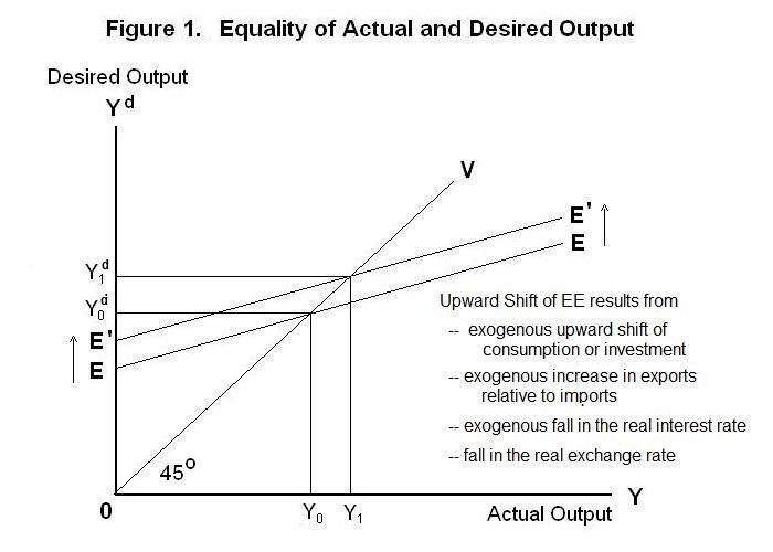
The equilibrating process can be seen with reference to Figure 1.
We now begin a more general analysis the overall equilibrium of a
small open economy. This equilibrium has two components:
The EE curve gives the response of desired income to be produced by domestic resources to the actual income those resources produce---its slope equals (1 - s - m) and will be less than the slope of a 45 degree line through the origin as long as either or both of the marginal propensity to save s and the marginal propensity to import m exceed zero. For deviations of output around its full-employment level it is likely that EE will be quite flat. Equilibrium occurs when Yd = Y which will occur along the 45 degree line OV . The EE curve will shift upward in response to exogenous upward shifts of desired consumption or investment represented by increases in the parameters a and δ , exogenous increases in desired exports relative to imports represented by increases in ( ΦBT + m* Y* ) and exogenous declines in r*. These shifts in consumption, investment and net exports are called exogenous because they originate outside the equilibrating process. Changes in consumption, investment and imports that arise from the resulting changes in income are called endogenous because they are generated within the equilibrating process. Exogenous shocks drive the model from the outside while endogenous changes occur within the model as it moves towards its new equilibrium. A fall in the real exchange rate, whether exogenous or endogenous, will shift world demand onto domestic output, also causing the EE curve to shift upward.
Suppose now that the desired level of domestic savings increases---that is, desired consumption falls---or, alternatively, the desired level of world investment allocated to the domestic economy declines. The results are shown in Figure 2.
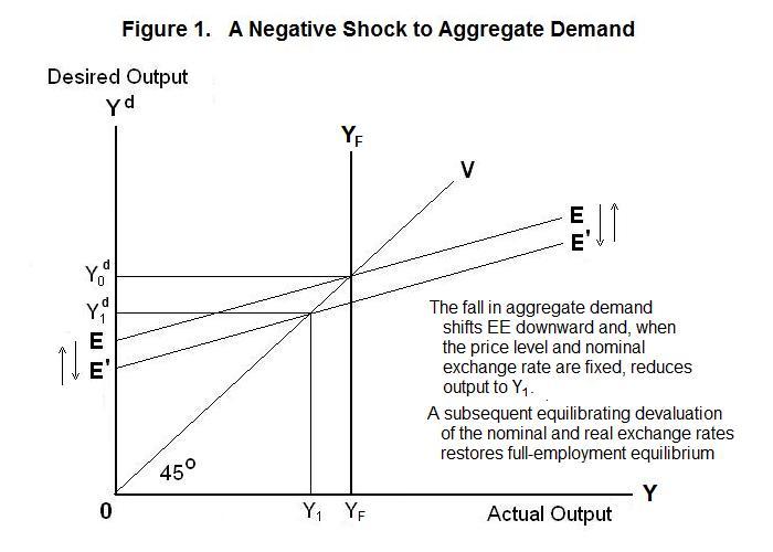
A reduction in desired consumption or investment reduces aggregate demand, shifting EE downward. If, in the short-run when prices are fixed, the domestic authorities maintain the nominal exchange rate constant, the equilibrium level of output falls below its full-employment level. If the authorities allow the nominal exchange rate to float, it will depreciate in response to the increase in the demand for foreign relative to domestic new capital expansion associated with the increase in desired domestic savings relative to investment. Since the domestic price level does not change in the short-run, the resulting reduction in the real exchange rate will shift world demand onto domestic goods, causing EE to shift back to its original level and the original full-employment level of output to be maintained. The details of this adjustment process will be expanded upon in the next and subsequent topics.
It is time for a test. As always, be sure to think up your own answers before looking at the ones provided.
Question 1
Question 2
Question 3
Choose Another Topic in the Lesson