The next step is to add the production possibility curve to our analysis.
This is done in Figure 1 below where the communities' production possibilities
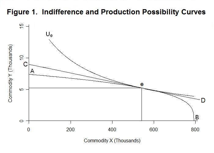
in our two-good world are represented by the curve running from point A to
point B. Using the production possibility curve together with an indifference
curve map enables us to venture into general equilibrium
analysis---that is, analysis of equilibrium in the economy as a whole as
opposed to concentration on that of a single industry or commodity. The
problem with such analysis, as we shall see, is that it involves an enormous
number of simplifying assumptions to avoid dealing with the myriad of details
of a complex economic system and thereby make the general equilibrium model
possible to solve.
The production possibility curve is convex outward from the origin because some of the economy's resources are better able to produce good X than good Y while other resources in the economy are better able to produce good Y than good X. A crude example of this would be one where two goods are being produced---food and housing. (Clothing is not necessary because, presumably, people in this economy run around naked all the time!) Different types of land are important for producing wood for homes as opposed to vegetables for food while labour is, say, equally important in the production of both food and housing. The more food that is produced, the greater the requirement for farm land, which becomes scarcer relative to demand and less productive at the margin. At the same time expansion of housing production, let us assume, simply involves cutting down more trees that grow in the wild in a forest that, say, replenishes itself naturally. Capital resources, can be assumed to be equally able to produce food or housing. If we were to start this economy out producing only housing, at point B in Figure 1, a small shift of labour and capital from housing production to food production will lead to a big expansion of food production associated with very little reduction in housing production since the best farm land can be used. So the production possibility curve increases dramatically as food begins to be produced. As the shift of resources from housing production to food production continues, however, it becomes necessary to use more and more labour and capital on poorer and poorer land with the result that the amount of food that can be obtained by sacrificing given quantities of housing gets smaller and smaller. So the negative slope of the production possibility curve gets smaller and smaller as production moves from point B to point A.
The optimal mix of goods X and Y for the economy to produce occurs at point e where, you will notice, the indifference curve is tangent to the production possibility curve. Since, as shown in the previous topic, the slope of the indifference curve equals the price of good X divided by the price of good Y, the slope of the production possibility curve at the equilibrium point where it equals the slope of the indifference curve must also equal the price of good X divided by the price of good Y.
In equilibrium under perfect competition, marginal cost equals price. This is the case because price represents the revenue to the firm from selling another unit while marginal cost is the increase in total cost from producing another unit. If price exceeds marginal cost the firm can increase its profits by producing and selling an additional unit. And if marginal cost exceeds price the firm can increase its profit by producing one less unit. All firms will therefore expand their output to the point where marginal cost and price are equal. In Figure 1, therefore, the slope of the production possibility curve at point e equals the ratio of the price of X to the price of Y, which must, since marginal cost equals price, be equal to the ratio of the marginal cost of good X to the marginal cost of good Y. And, since the price of X divided by the price of Y equals the ratio of the marginal utility of X to the marginal utility of Y, the socially optimum output mix occurs when
1. dTCx/dX / dTCy/dY = ∂U/∂X / ∂U/∂Y
where TCx is the total cost of good X and TCy is the total cost of good Y and the letter d in front of a variable denotes a small change in that variable, so that dTCx/dX is the marginal cost of good X and dTCy/dY is the marginal cost of good Y. As in the previous topic, ∂U/∂X and / ∂U/∂Y denote the respective marginal utilities of goods X and Y. Equation 1 gives an important condition for efficient allocation of resources in the economy---remember that the symbol ∂ denotes a small change with respect to the variable that follows, holding the other variable constant.
To model the whole economy on a two-dimensional graph such as Figure 1 in a completely rigorous fashion, we have to assume that all consumers are identical so that we can aggregate their preferences into a single utility function, and that all firms are identical so that their behavior aggregates into a single production possibility curve.
We can rather loosely interpret our conclusions, however, as also applying to a situation where the individuals are not identical but there is some coherent mapping of their combined preferences into a social utility function---the basis of this mapping would be that diminishing marginal utility holds for each good for each individual and that movements along the production possibility curve in the general neighborhood of point e do not involve major changes in the distribution of income across individuals. On the production side, we also have to assume that the different firms producing each good can be loosely aggregated in a way that yields a coherent production possibility curve for the economy. Moreover, to apply the analysis to an economy producing many goods we have to assume that the above two-dimensional graph can be extended to many dimensions and treat Equation 1 as applying to every pair of the many goods in the economy. The trick in doing economics is to simplify the analysis by imposing all assumptions that it is reasonable to believe will not significantly affect our conclusions while, at the same time, incorporating into our models all factors that will have important effects on the results. We can go wrong in two different ways: a) we can fail to assume away things that will not affect our results, making the analysis so complicated that we cannot sort out the major factors of importance; or b) we can assume away things that would, if included, have important effects on our conclusions, with the result that our conclusions become incorrect. Constructing a good theory thus requires making all the necessary assumptions and none of the unnecessary ones.
Our argument that point e in the above Figure gives the most efficient allocation of resources in the economy assumes that the indifference curves truly represent social preferences and that the production possibility curve represents the true social cost. And it also assumes that there is no difference between the price of each good paid by consumers and that received by producers and no difference between the marginal social costs of the individual goods and the private marginal costs of the firms producing them. We turn now to analysis of what happens when these assumptions do not hold.
Consider first the case where either the price received by producers differs from that paid by consumers or the marginal cost to producers does not reflect the social marginal cost. These situations essentially amount to the same thing---in both cases the ratio of the marginal costs of the goods to producers differs from the ratio of the marginal utilities of the goods to consumers. The consequences are a deviation of the mix of goods X and Y produced from the optimal mix as shown below in Figure 2.
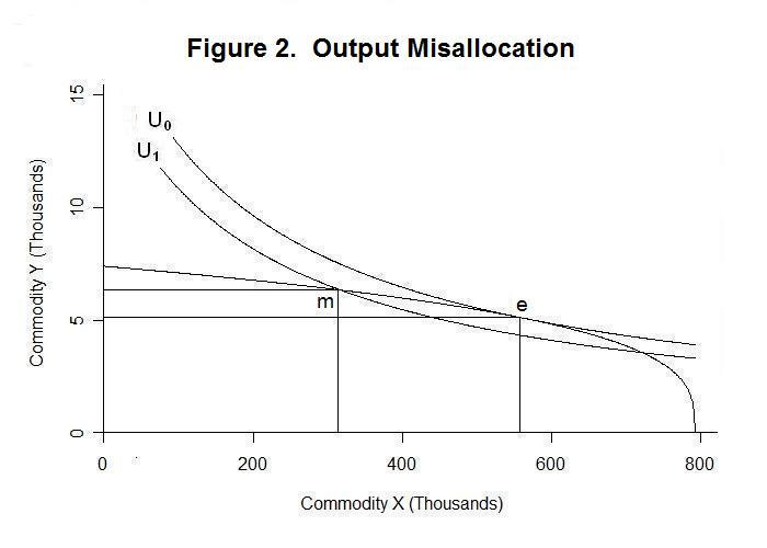
As was the case in Figure 1, the efficient mix is at point e. In Figure 2, however, the actual mix produced and consumed is at point m. Point e is optimal in the sense that the slope of the indifference curve (ratio of the marginal utility of X over the marginal utility of Y) is the same as the slope of the production possibility curve (ratio of the marginal cost of good X over the marginal cost of good Y). At point m, the slope of the indifference curve is steeper than the slope of the production possibility curve---the price of good X is higher relative to the price of good Y than it should be and the marginal cost of good X is lower relative to the marginal cost of good Y than it should be.
There are three broad reasons why the situation portrayed in Figure 2 might have occurred. First, the government could have put a tax per unit of output on good X but not on good Y. This will cause the price paid by consumers of X to increase relative to the price received by producers of that product. Output of good X will decline as the marginal cost declines along with the price received by its producers. The wedge between the price to consumers and the marginal cost of producers will cause the ratio of the marginal cost of good X to the marginal cost of good Y to fall relative to the ratio of the price of X paid by consumers to their price of good Y and, correspondingly, the ratio of the marginal utility of good X relative to the marginal utility of good Y. Notice here that to be completely rigorous in a two-good world we have to assume that the tax on good X is matched by a lump-sum transfer of funds to all consumers in a way that maintains the distribution of income unaffected---the government cannot be producing anything or we would have to add a third good. Our general conclusion, however, will probably apply in a broader situation where we assume government production constant in the background and the distribution of income basically unaffected by the imposition of the tax on good X rather than an appropriate lump-sum tax, which is the only type of tax which would itself not involve some resource allocation effect.
A second possible reason is that the production of good Y generates a cost, such as smoke or other atmospheric damage, that is external to the producers of the good. In this situation the price of good Y paid by consumers will equal the price received by producers producers but that price, and the marginal cost to producers of good Y will be less than the social cost of its production as a result of the externality, leading them to produce too much output. The indifference map incorporates all costs---i.e. disutilities---to consumers. So the price of Y will fall short of its marginal cost to society. As a result, the ratio of the social marginal cost of good X to the social marginal cost of good Y will be less than the ratio of the marginal utility of good X to the marginal utility of good Y. It is as if the government is subsidizing production of good Y by indirectly forcing the community to absorb a part of the social cost of producing that good---the price paid by consumers to producers of good Y does not completely cover the social cost of production. Of course, individual consumers as a group could eliminate the externality by simply reducing their consumption of good Y appropriately. It turns out, however, that the smoke-damage resulting from producing the amount any individual person consumes is so trivial in magnitude that the price he has to pay to consume a unit of the good does not reflect these costs. Everyone's utility is obviously diminished but this negative effect is the combined result of the aggregate production of good Y and not the quantity consumed by that person alone. For consumers to eliminate the externality, they would all have to agree to consume the output at point e and pay the price that will cause producers to produce that quantity of X.
A third possible reason could be the absence of perfect competition in the production of good X, a situation that will explored in detail in the three Topics that follow this one. To take the simplest case, suppose that there is a single producer of good X. When that producer expands output by one unit, the price of good X will fall so that the producer will receive less revenue from selling not only that last unit but all previously produced units. The producer's marginal revenue will thus be less than the price received. Since profit maximization occurs where marginal cost equals marginal revenue, the producer will produce less of the good than under a competitive situation where marginal cost equals price, making a monopoly profit as a result. Again, as illustrated in Figure 2, the ratio of the marginal cost of good X to the marginal cost of good Y (the slope of the production possibility curve will be less than the ratio of the marginal utility of good X to the marginal utility of good Y (the slope of the indifference curve).
The above three situations provide examples of the range of factors that can lead to a misallocation of the outputs of the goods produced relative to the socially preferred allocation. In these examples, the inputs used to produce the output mix are allocated so as to always produce the maximum output of each good, given the output of the other. Now it is time to relax this assumption, thereby allowing for a situation portrayed in Figure 3 below.
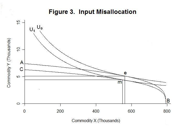
Suppose that the workers in firms that produce good Y become form a union and negotiate a significant increase in wages, while the market for labour in the production of good X remains competitive. To analyze the consequences, we need to look at the production process in more detail. The output of the firm depends upon the magnitudes of the inputs of labour and capital used to produce it. The relationship between inputs and output is given by the production function, which can be expressed in the case of only two inputs as
2a. X = F(Lx , Kx)
and
2b. Y = F(Ly , Ky)
in the cases of good X and good Y, where Lx and Ly are the quantities of labour used in producing the two goods and Kx and Ky are the quantities of capital. The marginal products of the respective inputs are the changes in output associated with small changes in each input, holding the quantity of the other input constant,
∂X/∂Lx = ∂F(Lx , Kx) / ∂Lx , ∂X/∂Kx = ∂F(Lx , Kx) / ∂Kx , ∂Y/∂Ly = ∂F(Ly , Ky) / ∂Ly and ∂Y/∂Ky = ∂F(Ly , Ky) / ∂Ky ,
where, as in the case of the marginal utilities, the symbol ∂ denotes a small change in the variable that follows, holding the quantity of the other input constant. Mathematically, the marginal products are the partial derivatives of the production function with respect to labour and capital. These marginal products are assumed to decline with an increase in the input and increase as a result of increases in the other input---that is, there is diminishing marginal productivity and increasing marginal cross-productivity.
Now consider the situation of a firm deciding how much of each input to use and how much output to produce. By using an additional unit of labour, for example, the firm increases its revenue by the marginal product of that unit multiplied by the price at which the unit of output can be sold---that is, by its value marginal product. At the same time, its costs increase by the wage rate paid to that unit of labour. If the value marginal product of labour exceeds the wage rate, the firm can increase its profit by employing an additional unit. It will continue to employ additional units until the value marginal product and the wage rate are equal. Should the wage rate exceed the value marginal product of labour, the firm will cut its output until the two become equal. Similarly, the firm will employ capital to the point where the value marginal product of capital equals its actual or implicit rental price.
We can now see what will happen when workers in the industry producing good Y form a union and negotiate a major increase in the wage rate. Individual firms can not afford to employ units of labour that cost more than their value marginal product---they will thus cut employment and production until the marginal product and value marginal product of labour has risen to the level of the union wage.
In the situation where all resources are devoted to the production of good X and good Y is not produced, the output combination will remain at point A in Figure 3 and the intersection of the production possibility curve with the X-axis will not change. In the other extreme case where only good Y is produced, output of that good will decline with a new production possibility curve crossing the y-axis at point C as compared to its original crossing at point A. Assuming that willingness to work increases with the wage rate, the quantity of labour employed will be less than the available supply at the union wage rate. The marginal product of labour and the value marginal product will be the same, although too high, in this situation because the price of the single good produced in the economy can be viewed as equal to unity.
It turns out that the new production possibility curve in Figure 3 will lie below the original one everywhere to the left of point B. To see this, consider the quantity of good Y produced associated with any particular output of good X. As an example, take the output of good X associated with the point e on the original production possibility curve. Under conditions of competition with many firms, the rental rate on capital will always adjust so that the entire capital stock will be employed. The immediate effect of the increase in the union wage in industry Y will be to cause the output of that good to decline for the reasons noted above. Labour will be released from the production of good Y and will enter the market for employment in producing good X pushing output of that good upwards. At the same time, however, the higher wage rate in industry Y will lead firms to substitute capital for labour in that industry, drawing capital from and reducing the output of industry X. By assumption, we are considering the case where the output of good X remains fixed, so that the movement of labour from industry Y to industry X and the movement of capital from industry X to industry Y must have equal effects on the output of X. The question is, what will be the net effect on the output of industry Y? The rise in the wage rate in industry Y clearly causes less output of that good to be produced and the value marginal product of labour in that industry to increase above the wage rate of labour in industry X. And the fact that labour moves to industry X and capital to industry Y in the case where the output of good X is unchanged will result in a decline in the value marginal product of labour in good X and an increase in the value marginal product of capital in X. And, of course, the decline in labour relative to capital in industry Y will reduce marginal product of capital there. Thus, at the price ratio and the quantity of X associated with the optimum point e, or any other point on the original production possibility curve to the left of point B, the value of total output could be increased by moving labour back from industry X to industry Y and capital back from industry Y to industry X in order to equate the value marginal products of each input in the two industries. The effect of the unionization of labour in industry Y must therefore have been to reduce the total value of national output at the original price ratio and must therefore have shifted the production possibility curve downward, reducing the quantity of good Y produced at any given quantity of X to the left of point B.
When we allow the output of X and relative output prices to adjust, the result will be a new equilibrium at point m at a lower level of output of both goods on a lower production possibility curve and a lower indifference curve, representing a reduction in social utility.
Our final application of indifference curve and production possibility curve analysis is to the gain from international trade. We proceed with reference to Figure 4 below where, in the absence of trade, the country produces X0 of good X and Y0 of good Y, with equilibrium at point a on indifference curve U0. The ratio of the price of X to the price of Y will equal the equivalent slopes of the indifference curve and the production possibility curve at point a.
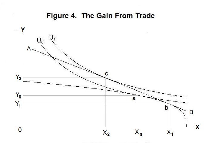
Suppose now that the price of good Y relative to that of good X, given by the inverse of the slope of the line A B in the above Figure, is much lower in the rest of the world than in the domestic economy in the absence of trade. Domestic residents can import good Y much cheaper than they can produce it at home, and obtain a higher price for their output of good X in the world market than in the domestic economy. They can thus increase their production of good X from X0 to X1 and reduce their production of good Y from Y0 to Y1 and then sell the quantity (X1 − X2) abroad in return for the quantity (Y2 − Y1) of good Y. The equilibrium output mix will thus shift from point a to point b and the equilibrium mix of the two goods consumed will shift from point a to point c, putting the society on the higher indifference curve U1. By engaging in international trade, the country's residents can consume a mix of goods X and Y outside their domestic production possibility curve.
While this analysis clearly demonstrates the gain from trade, it does not incorporate the distribution effects that ultimately result from a real-world movement to free trade. The indifference curves properly incorporate the utility of domestic residents as consumers but do not include redistributions of utility resulting from the movement of labour and capital from the production of good Y to the production of good X. Workers living in the area of the country producing good Y will have to move to the area where the production of good X is taking place. Unless the gainers from free trade compensate them sufficiently they will try to prevent the movement to free trade, demanding protection for their industry. What the analysis does clearly show, however, is that the gainers from international trade can compensate the losers sufficiently for everyone to be better off. While distribution effects were also clearly present in the analysis of union imposed wages in our earlier analysis, that was a case where the gainers could not compensate the losers and still be better off.
Again, it is time for a test. Be sure to think up your own answers before looking at the ones provided.
Question 1
Question 2
Question 3
Choose Another Topic in the Lesson