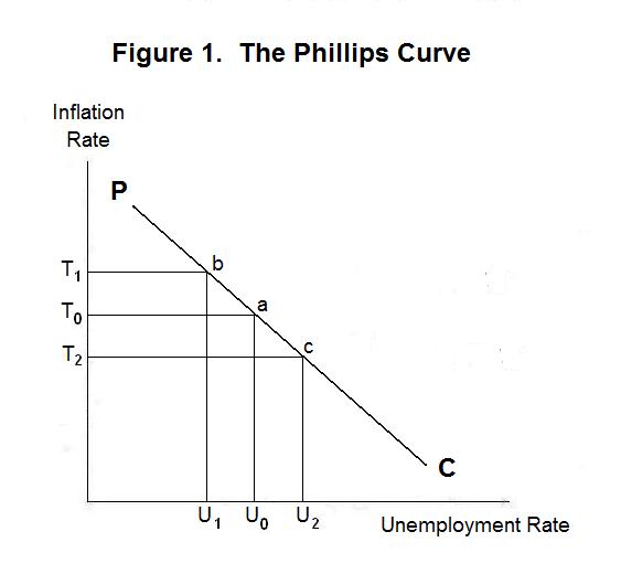
Although Phillips' original paper related the rate of growth
of nominal wage rates to the unemployment rate, it has become
customary to express the Phillips curve a relationship between
the inflation rate and the unemployment rate, as shown by the
curve PC in Figure 1. The inflation rate is on the vertical axis
and the unemployment rate on the horizontal axis.
In 1958, A. W. Phillips (1914-1975) published an important
paper that found a significant negative relationship between the
rate of increase of nominal wages and the percentage of the
labour force unemployed during important periods in British
economic history. This relationship, which came to be called
the Phillips Curve, suggested that government could reduce the
unemployment rate by creating a more rapid rate of inflation of
wages and prices. The basis for and validity of this apparent
trade-off between inflation and unemployment is the focus of
this Topic.
The rationale for a negative relationship between the rate of inflation and the unemployment rate in the short-run is easily seen from the analysis in the preceding Topics in this Lesson. An unexpected expansion of the nominal money supply or decline in the demand for money will increase the long-run equilibrium price level. Workers and firms, unaware that the aggregate demand for output has increased, will increase wages and prices by less than will be required for equilibrium to be achieved. As a result, output and employment will increase above their full-employment or natural levels.
As long as some price level response to the increase in aggregate demand occurs, the rate of inflation will increase as the unemployment rate declines. In Figure 1, the unemployment rate falls to U1 and the inflation rate rises to T1 with the inflation-rate, unemployment-rate combination moving from point a to point b . Similarly, an unanticipated decline in the money supply or increase in the demand for money will cause the price level to fall, albeit more slowly than it should, and the rate of unemployment to increase, as shown by the movement of the inflation-rate, unemployment rate combination from point a to point c.
It is straight-forward to argue that by increasing the rate of money growth and the equilibrium inflation rate, the authorities can induce a reduction in the unemployment rate as workers and firms adjust wages and prices with a lag and the excess demand spills over onto aggregate output. In the 1960s and early 1970s many economists believed that society faced a tradeoff between inflation and unemployment---by tolerating (creating) a higher inflation rate the authorities could engineer a reduction in the unemployment rate. Since unemployment is worse than inflation, an increase in the inflation rate seemed to be a useful cost to bear in promoting a good cause.
It should be obvious from what you have learned in the first three Topics of this Lesson that obtaining a long-run reduction the unemployment by generating a higher inflation rate is an illusion. Once workers and firms realize that the equilibrium rate of inflation has increased they will increase wages and prices by that equilibrium amount and full-employment will be continuously reestablished. The reduction in the unemployment rate occurs because wage and price setters are misinformed about the state of aggregate demand and fail to increase wages and prices fast enough. Once they learn what is happening workers and firms will adjust wages and prices to fully compensate for the inflation they know is occurring. At that point, unemployment will return to and remain at its natural rate.
To reduce the unemployment rate beyond the short-run, the authorities have to create a further increase in the inflation rate whenever wage and price setters come to anticipate the last increase, and then further again escalate the inflation rate when that increase has become fully anticipated, and so forth. But this too will fail because wage and price setters will come to realize that the government is increasing the equilibrium rate of inflation rate at an accelerating rate and will respond with an equivalent acceleration in the rate at which they increase wages and prices.
The situation can be analyzed with respect to Figure 2. Suppose that the authorities increase the inflation rate from T0 to T1 and maintain it there. At first workers and firms, not realizing how much the equilibrium inflation rate has risen, increase wages and prices by too little, with the result that the unemployment rate falls to U1 at point b. As time passes, and wage and price setters realize what is happening, however, they appropriately increase wages and the unemployment rate returns to U0 at the maintained inflation rate T1 as indicated by point c. The long-run result is an increase in the inflation rate with no reduction in unemployment.
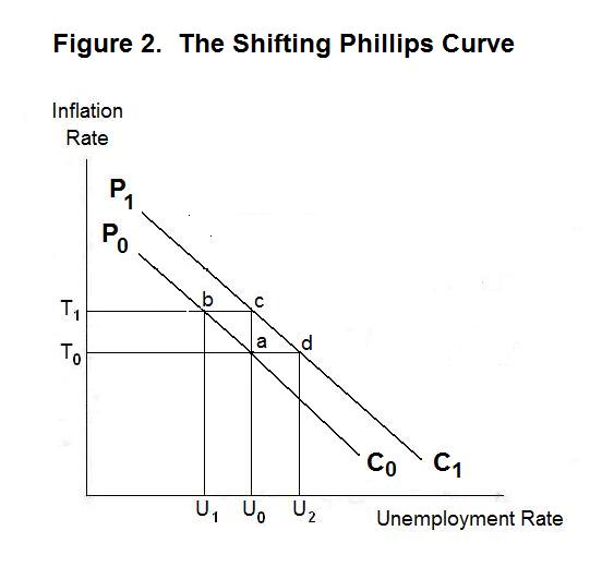
The level of the Phillips curve thus depends on the expected rate of inflation. When the expected rate of inflation rises from T0 to T1 the curve shifts up from P0C0 to P1C1. The natural rate of unemployment U0 is then associated with the higher equilibrium inflation rate T1. The government can temporarily reduce the unemployment rate along this new Phillips curve by unexpectedly increasing the equilibrium rate of inflation, but as soon as workers and firms realize what has happened the Phillips curve will again shift up and the unemployment rate will return to U0.
Government policy makers do not face a tradeoff between inflation and unemployment in the long run. And, though they face a short-run tradeoff, any attempt to exploit it will ultimately result in a permanent increase in the inflation rate. Moreover, once that permanent increase in the inflation rate has occurred, the government will only be able to eliminate it at the cost of an increase in unemployment above the natural rate. For example, suppose that in Figure 2 the government lowers the equilibrium inflation rate from T1 to T0. Until workers and firms realize what has happened the unemployment rate will rise to U2 at point d . The authorities could prevent this increase in unemployment if they could convince workers that they really are going to lower the equilibrium inflation rate to T0. But the government has an incentive to lie to wage and price setters. If it can convince them that it is going to lower the equilibrium inflation rate to T0 so that the Phillips curve shifts down to P0C0, and then renege on that commitment, the political party in power will take credit for a reduction of the unemployment rate from U0 to U1. Such deception can be irresistible when the next election is within sight.
Because of the problem of credibility, it turns out to be very difficult for governments to reduce their countries' inflation rates without causing temporary increases in unemployment rates. As a result, the short-run tradeoff of inflation for unemployment cannot be usefully exploited if inflation is to be controlled in the long run.
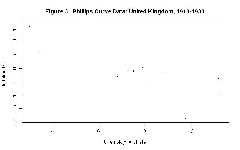
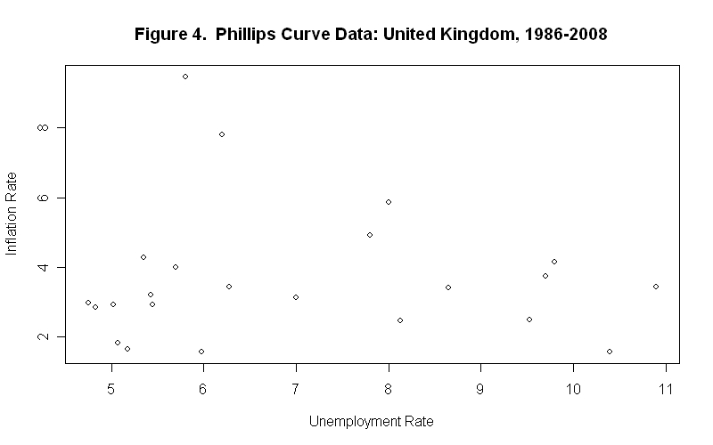
In concluding this Topic we examine some of the evidence on the Phillips curve. Figure 3 clearly suggests a Phillips curve for Great Britain during the period 1919-1930, but Figure 4 shows little evidence of a negative relationship between the British inflation and unemployment rates for the period 1986-2008---it turns out that an Ordinary Least Squares (OLS) regression in fact indicates a negative relationship for which the P-Value (probability that the observed relationship could occur on the basis of pure chance) is slightly more than 1 percent, but the R-Square (fraction of the variance in the inflation rate explained by the unemployment rate) is only .16.
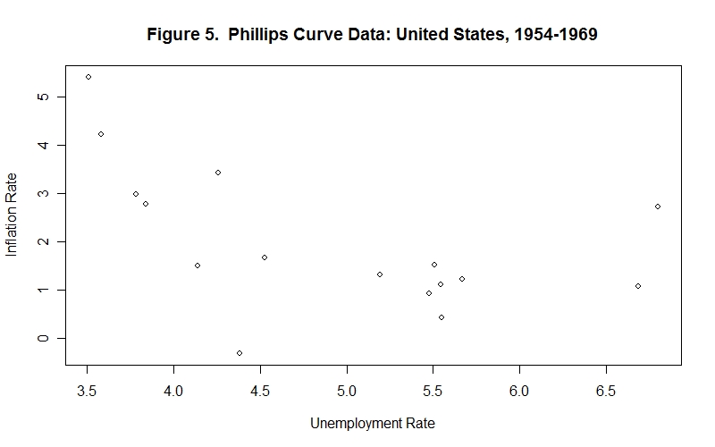
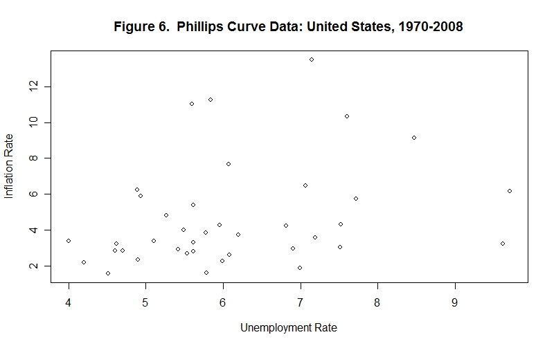
While a rough negative Phillips-curve relationship for the U.S. for the years 1954-1969 appears in Figure 5, although the P-Value is slightly more than 5 percent and the R-Square is only .28, there is clearly no negative relationship between the inflation and unemployment rates in the period 1970-2008 in Figure 6 where the underlying OLS regression line has a positive slope.
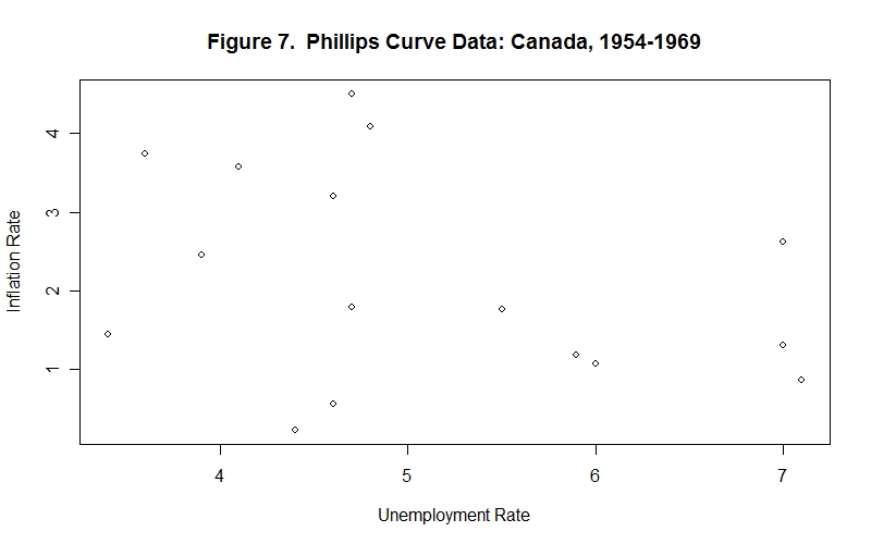
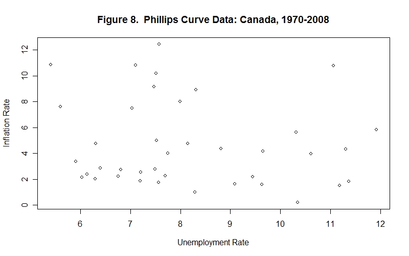
For Canada we cannot observe a coherent Phillips curve relationship in the data for either 1954-69 in Figure 7 or 1970-2008 in Figure 8. It turns out that the OLS regression lines are negatively sloped in both periods, but the P-Value is higher than 20 percent and the R-Square is only .11 in the earlier period and in the 1970-2008 period the P-Value is 44 percent and the R-Square is .015.
It is obvious that the Phillips curves for the United Kingdom, the United States and Canada were shifting during the periods examined---this accounts for the weakly negative, and often positive, relationships observed in the data.
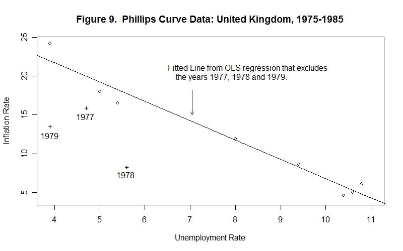
Finally, the data for Great Britain for the period 1975-85 are particularly interesting. As shown in Figure 9, the inflation-rate, unemployment-rate combinations for the years 1975-76 and 1980-85 seem to lie on the same Phillips curve. An OLS regression line obtained for these years is shown on the graph---the P-Value for the negative slope, is .00146 percent, indicating that the likelihood of obtaining a negative slope by random chance is less than 2 times in a thousand. The two years 1978 and 1979, and to a lesser extend 1977, are outliers which suggest that wage and price setters were temporarily fooled by the abortive 1977 inflation reduction effort (undertaken in connection with a loan from the International Monetary Fund) into believing that the high inflation rate would decline.
It is again time for a test! As always, think up your own answers before looking at the ones provided.
Question 1
Question 2
Question 3
Choose Another Topic in the Lesson