For subsequent illustrative numerical calculations, the industry demand
curve in the four-firm case is represented by the linear function
1. P = 70 − 0.01625 Q .
where Q is the industry output. Under complete collusion, with the firms
of equal size so that Q = 4 q , each individual firm's
demand curve is again, as in the duopoly case, equal to
2. P = 70 − 0.065 q
and its marginal revenue curve is again
3. P = 70 − 0.13 q .
The individual firms cost curves are also exactly the same as in the previous
Topic. All numerical calculations are now performed in the program R using
the input file cournot.R to generate the resulting
output file cournot.Rou.
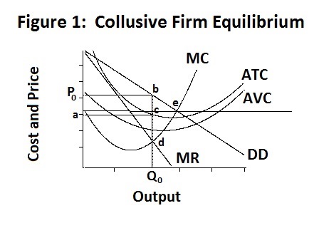
The equilibrium of the individual firm under collusion is portrayed in
Figure 1, which is identical to the corresponding Figure in the previous
Topic, with the equilibrium industry output now being four times the individual
firm's output.
Our task now is to extend the analysis of the previous Topic to the case of
oligopoly where there are a limited number, but more than two, firms. We begin
by assuming that there are four firms, each identical to the
firm examined in the last Topic in terms of costs and share of the industry
demand---this will imply that the industry is twice as large as the one
analyzed in the duopoly case. The analysis will subsequently be extended to
incorporate ten firms.
Again, each firm produces 435 thousand units of output at an average total cost per unit of $29.80 and a selling price of $41.73, earning excess profits of 5187.85 thousand dollars. The equilibrium occurs where every firm's collusive marginal revenue equals its marginal cost at point d , with excess profits per unit equal to b c .
The socially efficient output occurs where the firm's marginal cost equals the price, at point e in the figure above. This efficient equilibrium can only be achieved with government regulation whereby the price is fixed so that the individual firm's demand curve is the horizontal dashed line through point e . Since price is above average total cost at that equilibrium output, all four firms will earn excess profits, although these profits are too small to permit entry of a fifth firm. Our numerical calculations indicate that each firm will produce an output of 583 thousand units at the regulated price of $32.105 and the average total cost of $28.003, earning excess profits of 2390.986 thousand dollars. These profits can be taxed away by the government in lump-sum form.
The more interesting case is where there is no government regulation and one firm decides to break away from the agreed-upon collusive equilibrium. This situation is portrayed in Figure 2 below. Here the line DD gives the demand curve and MR the marginal revenue curve of the break-away firm, assuming that all other firms produce the collusive output levels. Since the firm represents one-quarter of the industry, the slope of its demand curve will equal −0.01625 , the same slope as the industry demand curve presented in Equation 1. The DD line thus passes through the collusive price quantity combination and the firm produces the output Q1 . The collusive demand and marginal revenue curves are given by the dotted lines that intersect the price axis at point h .
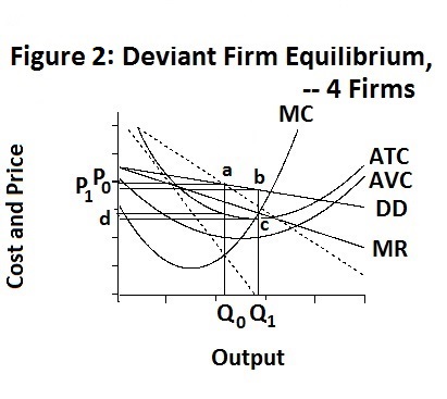
The above equilibrium occurs where the firm's marginal cost curve, given by MC , crosses its marginal revenue curve yielding excess profits given by the rectangle P1 b c d . Our numerical calculations indicate a new market price equal to $41.73 and output level of 572 thousand units produced at an average total cost of $29.80, yielding an excess profit of 6614.273 thousand dollars which is 1426.326 thousand dollars more than the firm's profit when it abides by the collusive arrangement. Each of the three other firms, which are assumed to maintain their outputs at the collusive level, lose 968.42 thousand dollars, resulting in a loss of the four firms combined equal to 1490.73 thousand dollars due to the deviant behaviour of the one firm.
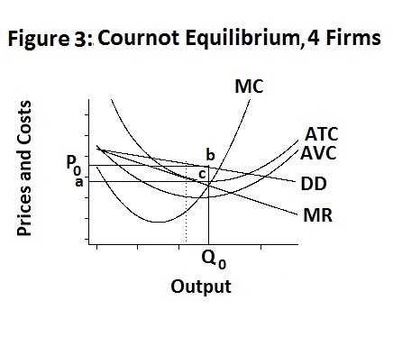
It makes no sense, of course, for the other three firms to maintain a collusive arrangement under these circumstances so they too will each deviate in the most profitable manner given the other firms' behaviour. The result will be the Cournot equilibrium portrayed in Figure 3 below.
Each firm adjusts its output to maximize its profits, which are equal to
4. π = P(Q) q − C(q) ,
where π is the individual firm's profit, Q is the level of industry output, q is the level of output of the individual firm where all firms are assumed to be identical, C(q) is the individual firm's total cost curve and P(Q) is the industry demand curve given by Equation 1. Each firm adjusts q until π is at its maximum, at which point
5. dπ/dq = P(Q) + q dP(Q)/dq − dC(q)/dq = P(Q) + q dP(Q)/dQ dQ/dq − dC(q)/dq = 0 .
This expression can be rearranged to yield the equality of marginal revenue with marginal cost
6. P(Q) + q dP(Q)/dq = dC(q)/dq ,
where dQ/dq = 1 . Substituting Equation 1 and noting that dP(Q)/dq = 0.01625 , the expression for marginal revenue becomes
7. MR = 70 − (0.01625) (.75 Q) − 0.01625 q
The term 70 − (0.01625) (.75 Q) gives the intersection of the individual firm's demand curve with the price axis. This demand curve shifts down as the other three firms expand their output.
Equilibrium occurs where MR , the marginal revenue curve associated with the individual firm's demand curve crosses the firm's marginal cost curve MC . The individual firms' average total costs at that output are given by the distance between point c and the quantity axis, with the result that each firm earns excess profits equal to the rectangle P0 b c a . The vertical dotted line gives the firm's output under complete collusion as compared to the higher cournot output Q0 .
The numerical results in cournot.Rou indicate that under Cournot equilibrium each firm produces 543 thousand units of output at an average total cost of $27.96 and sells that output at a price of $34.70 , earning a profit of 3660.056 thousand dollars. This is 1527.79 thousand dollars less than the 5187.847 thousand dollars that the firms could individually earn under complete collusion.
Of course, this Cournot equilibrium can also be viewed as a Nash equilibrium in a four-firm game but the solution of that game is too technically complicated to merit a venture into the game-theory analysis involved at this time.
Finally, we can extend the analysis to incorporate ten oligopolistic firms rather than just four, assuming that under collusion their outputs are the same as in the four-firm case, with the industry being two-and-one-half times as large. In this case the collusive profits of each firm are the same as before with a deviant firm now producing an output of 609 thousand units and increasing its profits to $7530.478. Under a cournot equilibrium shown in Figure 4 below, each firm earns a profit of $3612.852 thousand, given by the rectangle P0 b c a . and produces an output of 567 thousand units.
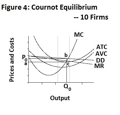
It is interesting to note that as the size of the industry and the number of firms increases the cournot demand curves get flatter and the marginal revenue curves become closer to them with the results becomming closer to those under monopolistic competition.
It is test time. Do yourself an intellectual favour by working up your own answers before looking at the ones provided.
Choose Another Topic in the Lesson