It is now time to investigate more thoroughly the factors
determining the shape of the supply curve. The supply curve can
be visualized in two ways---as the response of the
quantity supplied to variations in the price, or alternatively,
as the response of costs of production and sale as the quantity
sold changes.
When there is competition among suppliers, the prices of
goods supplied will be bid down to levels that will just cover
costs including reasonable returns to capital invested and
entrepreneurial effort expended. The analysis of the relations
between the quantity supplied and the price at which it will be
supplied therefore depends critically on how costs behave as the
quantity produced and sold increases.
When more output is produced and sold, more labor, capital
and other inputs must be used to produce that output. These
inputs must earn a return or wage to compensate their owners for
their use. Costs will rise if higher wages have to be paid for
these inputs as additional quantities of them are employed, or
if successive applications of these inputs are less and less
effective in producing output. This latter situation is called
diminishing returns.
Diminishing returns is an important feature underlying many
supply curves. Consider, for example, the supply curve of an
agricultural product such as corn. As the quantity produced
increases additional quantities of machinery, fertilizer and
labor must be applied to a fixed available stock of land. As
more and more of these inputs are applied to the land the
additional output that can be obtained from additional units of
the inputs gets smaller and smaller. Yet the most recently
applied units of these inputs cost the same as those units that
were applied earlier when the level of output was smaller. The
cost per unit of output thus increases as more and more output
is produced. Suppliers must receive a higher price to induce
them to produce additional units of output. This is shown in the
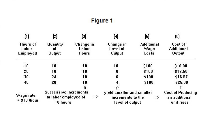
tabular presentation in Figure 1.
A product is produced with the application of labor hours to a given quantity of land. As labor is added in 10 hour increments (columns 1 and 3) output increases in successively declining increments---10, 8, 6, 4 (columns 2 and 4). At an assumed wage rate of $10 per hour, each increment of labor hours costs $100. This means that the first 10 units of output cost $10.00 each to produce, the next 8 units cost $12.50 each, the next 6 units cost $16.67 and the last 4 units cost $25.00. Successively higher output prices are thus required to call forth additional supply.
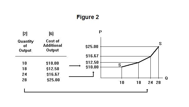
The tabular material in Figure 1 is presented in Figure 2 in the form of a supply curve. Column 2 gives the quantity of output, which is shown on the horizontal axis, and Column 6 gives the cost of additional output, which is equated with the price necessary to get the producer to supply that additional output, shown on the vertical axis.
It is not the case, however, that all supply curves are conditioned by diminishing returns. Consider, for example, the supply curve of TV sets. This product is produced with many different kinds of labor and capital but no land. Producers of TV sets can hire additional labor away from other activities at the going market wage and additional new capital can be installed in the industry producing TV sets at no greater costs than required for previous capital---additional inputs are simply put to work in the TV industry rather than somewhere else at the same cost. Since the production of TV sets uses a very small fraction of the total stock of these particular inputs in the economy as a whole, the cost per unit of output of TV sets is not likely to rise noticeably as that output expands. The supply curve of TV sets is therefore likely to be a horizontal line. Industries like this are called constant cost industries. Agriculture, mining, forestry and other natural resource industries that face diminishing returns are called increasing cost industries. Some industries also exist for which costs decline as output increases. These are decreasing cost industries. The reasons for decreasing costs will be discussed later. The supply curves of these three types of industries are illustrated in Figure 3.
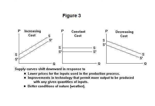
The factors causing supply curves to shift are also outlined in the above Figure. A movement along the supply curve occurs as costs per unit respond to increases in the quantity supplied. These costs are affected by the prices that producers must pay for labor and capital inputs. A rise in the prices of these inputs that occurs as a result of an expansion of output will cause the supply curve to become steeper. A rise in the prices of these inputs that is independent of output in this industry will cause the supply curve to shift upward---costs will increase at each level of output. A fall in input prices independently of industry output will cause the supply curve to shift downward as illustrated by the movements from SS to S'S' in Figure 3.
The supply curve will also shift in response to technological changes affecting the industry. A improvement of technology implies that each level of output can be produced with less labor and capital inputs than were required previously. This means that costs per unit of output fall at each level of output, shifting the supply curve down.
Finally, there is the effect on supply of natural forces such as weather. Better weather means better crops with the result that more output will be produced for any given application of labor and capital inputs. This will shift the upward sloping supply curve for agricultural output to the right---viewed alternatively, it means that each output level can be produced at lower cost with the result that the supply curve can be thought of as having shifted down.
It is now time for a test. As always, think up an answer of your own before looking at the one provided.
Question 1
Question 2
Question 3
Choose Another Topic in the Lesson.