In order to raise revenue to finance its expenditures,
the government frequently finds it useful to tax particular
commodities. Sometimes the tax is levied on the consumer,
requiring that the consumer pay the government, say, T dollars
for every unit of the good bought. Sometimes the tax is levied
on the producer, requiring that she pay the government $T for
every unit sold. We can show that, despite superficial appearances, it may
make no difference whether a given tax is levied on the consumer or
the producer.
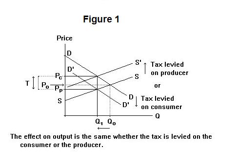
Figure 1 portrays the situation for a typical commodity that
might be taxed.
The initial pre-tax equilibrium is the price-quantity combination ( P0 , Q0 ). Suppose that the government imposes a tax on the consumer of the good equal to T dollars per unit consumed. The consumer now has to subtract $T from the price he is willing to pay the producer for each quantity of the good---her demand curve therefore shifts downward from DD to DD'. Producers' costs, and hence the supply curve, are unaffected. As a result of the leftward shift of the demand curve, the equilibrium quantity will fall from Q0 to Q1. The consumer pays the price Pc, the producer receives the price Pp, and the government takes the difference Pc − Pp as tax.
Suppose alternatively that the tax of $T per unit is levied on producers, who now have to give the government $T for every unit they sell. At each output level producers now have to charge consumers a price $T higher to cover their costs---their supply curve thus shifts up by $T as shown by the curve S'. In this case, the demand curve is unaffected. The equilibrium quantity again falls from Q0 to Q1. Again, consumers end up paying the price Pc, producers receive the price Pp, and the government takes the difference Pc − Pp as tax.
A tax on a commodity can be viewed simply as driving a wedge between the price paid by the consumer and the price received by the producer. This is shown in Figure 2.
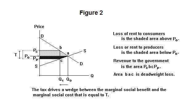
Pc is the price paid by the consumer and Pp is the price received by the producer. The consumer surplus or rent is reduced by the shaded area above the price P0. The producer surplus or rent is reduced by the shaded area below the price P0. The total loss of rents to both consumers and producers is thus the area Pc b a c Pp. But the rectangle Pc b c Pp is not lost to society---it simply goes to the government as tax revenue, to be spent on goods and services that are, at least in principle, beneficial to society. It is a redistribution of income from those who pay the taxes to those who get the benefits of the government's expenditure of those funds. The triangle b a c represents an efficiency loss to society. When consumption is at Q1, consumers would be willing to pay the price Pc for an additional unit of the good. That additional unit of the good would cost society Pp. Society would be better off if the additional unit were produced and consumed. But it does not pay producers to produce it because its after-tax price is below their cost of production. All the the units of output between Q1 and Q0 would similarly benefit society if it would pay producers to produce them.
Output levels below Q0 are inefficient because the marginal social benefit from producing another unit at these output levels is greater than the marginal social cost. Producers and consumers operate where their marginal private benefits are equal to their marginal private costs. Output cannot expand beyond Q1 because the marginal private and social benefit Pc, which equals the marginal private cost ( Pp + T ), is greater than the marginal social cost Pp. Marginal private costs are thus above marginal social costs by the amount of the tax.
The incidence of a tax---that is, the proportions of the tax revenue ultimately paid by consumers and producers---is independent of whether it is consumers or producers that have to pay the tax to the government. What determines the actual incidence of the tax is the slope of the demand curve relative to the slope of the supply curve. Consider, for example, Figure 3.
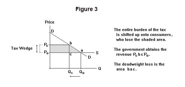
The supply curve is horizontal and the marginal social cost is independent of the quantity sold. Producers receive no rent in the pre-tax situation and lose none as a result of the tax. Consumers, on the other hand lose the shaded area. Of this, the area Pc b P0 is tax revenue to the government, to be used to provide equivalent benefits to the society in the form of government services. The area b a c is deadweight efficiency loss. Were consumers to consume Q0 rather than Q1, they would receive total benefits equal to the area b Q0 Q1. The cost to society would be the area c a Q0 Q1, leaving a net social benefit of a b c. Consumers cannot capture that benefit because the marginal private cost of the good to them is equal to P0 plus the tax and is therefore above the social cost P0.
In Figure 4 below, the demand curve is perfectly elastic and the supply curve is upward sloping.
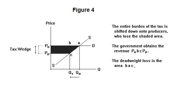
The burden of the tax is thus shifted down onto producers. Consumers received no surplus as a result of buying from these producers in the pre-tax situation and they lose none as a result of the imposition of the tax. This might be a situation where producers are selling on the world market at a fixed price. Consumers may earn rents from consuming the product, but none of those rents arise because of purchases from domestic producers---they can buy all they want elsewhere at a fixed price so they will never pay more than that price to domestic producers. The price received by domestic producers thus falls by the amount of the tax. Note that this tax must be levied only on sales of the domestic product if Figure 4 is to apply. If it were levied on purchases by domestic consumers from all sources they would have a situation described in Figure 3. Consumers would be buying a tiny share of the world supply and would be able to purchase all they want at the fixed world price. Producers would be able to sell all they want at a fixed price, so their situation would be described by Figure 4.
When the tax is levied on purchases of domestic product, the price to the consumer remains equal to the world price while the price to the producer has to fall by the amount of the tax. Producers lose rents equal to the shaded area in Figure 4. Of this, the area P0 b c Pp is tax revenue to the government, to be beneficially used elsewhere and the area b a c is efficiency loss. The marginal private and social benefit from domestic production is P0 while the marginal social cost is Pp. Since the marginal private cost is P0 ( = Pp plus the tax ) , the output produced will be too low---the marginal private cost, which equals the marginal private and social benefit, is greater than the marginal social cost.
It is possible for the tax to be shifted entirely onto the producers even if the demand is not perfectly elastic. This is illustrated in Figure 5 where the supply curve is vertical and the demand curve exhibits the usual negative slope. Because the supply curve is vertical, the marginal social and private costs of producing all outputs up to and including Q0 are zero. Since producers will produce quantity Q0 regardless of the price, the quantity produced is unaffected by the tax. Competition among consumers will maintain the market price at P0 and the net-of-tax price received by producers will fall to P0 minus the tax.
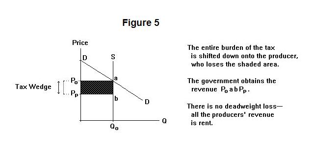
The case portrayed in Figure 5 is an example where all the revenue to suppliers is rent and, according to the definition of rent, can be taxed away by the government without any effect on output. There is thus no deadweight or efficiency loss.
The analysis above seems to suggest that commodity taxation is often bad because it reduces efficiency. Commodity taxes are indeed inferior to what economists call neutral taxes---those that have no efficiency effects. Unfortunately, every tax that can, in practice, be levied has an adverse efficiency effect of some kind. The problem then becomes one of choosing taxes that have, along with other desirable properties, the least adverse effects on economic efficiency.
It is time again for a test. Think about your answers carefully before looking at the ones provided.
Question 1
Question 2
Question 3
Choose Another Topic in the Lesson.