The equations of asset and goods market equilibrium that were developed
the previous topic are reproduced here as Equation 1 and Equation 2
below with the domestic real interest rate determined at the level
r* by conditions in the world market.
1. r*
= − (1/θ) M/P + γ/θ −
τ + (ε/θ) Y
2. Y
= ( a + δ
+ ΦBT + DSB)/(s + m)
− μ/(s + m) r
+ m*/(s + m) Y*
− σ/(s + m) Q
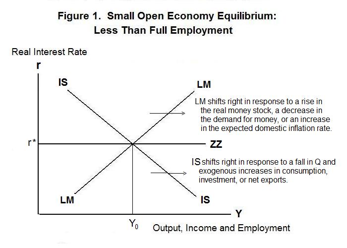
The IS curve in Figure 1 gives the combinations of income
and the world-determined real interest rate for which the aggregate quantity
of domestic output that world residents wish to purchase equals
the quantity produced. An increase in the real interest
rate causes a reduction in desired domestic investment leading to
an upward movement along the curve and a decline in real income.
A rise in the real exchange rate shifts domestic and foreign
demand off domestic goods causing the desired current account
balance to deteriorate and the IS curve to shift to the left---a
smaller level of domestic income is now associated with each
level of the world interest rate. An exogenous increase in
desired consumption or investment, increase in desired exports,
or reduction in desired imports shifts IS to the right.
The small open economy is in equilibrium when both stock
(asset market) and flow (real goods market) equilibrium hold.
The process of getting to equilibrium will depend upon whether
the nominal exchange rate is fixed by the government or allowed
to float freely in response to the forces of supply and demand.
It will also depend on whether prices are flexible and the economy
is fully employed or the price level is institutionally rigid and
unemployed labour is present. At this point we assume that the exchange
rate is flexible, the price level is fixed and there is less than
full employment in the economy.
The LM curve in Figure 1 gives the combinations of income and the world-determined real interest rate for which desired money holdings equal actual holdings and, hence, desired aggregate non-monetary asset holdings equal actual holdings. A rise in the real interest rate, holding M/P constant, reduces desired money holdings and requires an increase in income to increase them back to their initial level---the LM curve is positively sloped. An increase in the real money supply (increase in M or fall in P) requires a higher level of real income to produce an equivalent increase in desired money holdings at a constant world interest rate---LM thus shifts to the right. An exogenous increase in desired real money holdings has the opposite effect. An increase in the expected inflation rate reduces desired money holdings at each level of r* and Y , shifting LM to the right.
When the domestic price level is fixed and there is less than full employment all real exchange rate adjustments must fall on Π . Since P cannot change, and the real interest rate is determined by world market conditions, the only way that asset equilibrium can be maintained is through changes in domestic income and employment. The less-than-full-employment equilibrium level of domestic income will then be that level for which domestic residents are willing to hold the existing money supply at the world-determined interest rate. This will be the level of income at which LM crosses the horizontal line ZZ.
All this can be seen by looking at Equation 1, the equation of asset equilibrium. M is fixed by the government, P is fixed by short-run wage and price rigidity, r* is fixed by world market conditions, and τ is determined by people's expectations based on past history. The only variable in Equation 1 that can change to produce equilibrium is Y .
Now look at the real goods market equation, keeping in mind that Y is determined in the Equation 1, the asset market equation. Foreign income, Y* and r* are determined in the rest of the world and the only variable that can adjust to maintain real goods market equilibrium is Q . And since P is fixed, all adjustments of Q must take place through changes in Π . This means that the level of income will be determined at the point where LM crosses ZZ, and that the nominal exchange rate must continually adjust to ensure that the IS curve crosses through that same point.
To visualize this adjustment process, consider Figure 2. Imagine a government policy induced increase in the money supply or an exogenous decrease in domestic residents' demand for money. The LM curve shifts to the right to LM'. Domestic residents try unload their excess money balances and reestablish portfolio equilibrium by purchasing assets from foreign residents, creating an excess supply of the domestic currency on the foreign exchange market. This causes the domestic currency to depreciate. Given that Q = P / Π P* , Π will rise, switching world demand onto domestic goods and shifting the IS curve to the right. The resulting increase in output, employment and income as commodity market equilibrium is maintained raises domestic residents' desired money holdings. This adjustment process will continue until IS crosses LM' on the ZZ line at income level Y1.
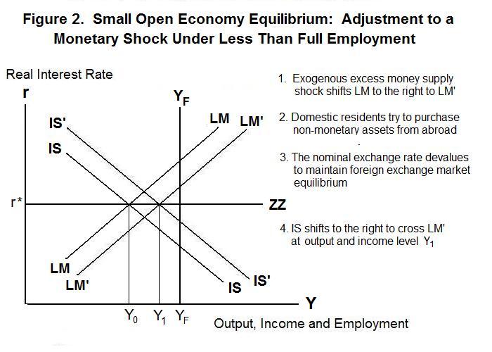
In the example above, the shock to monetary equilibrium shifts LM to the right, inducing a fall in the real exchange rate sufficient to bring about an equivalent rightward shift of IS. This is the essential principle of small-open-economy equilibrium under flexible exchange rates. Equilibrium output is determined by LM and ZZ ---that is, by the condition of asset equilibrium at the interest rate determined by world market conditions. Goods market equilibrium occurs automatically through nominal exchange rate adjustments which ensure that IS will cross through the LM-ZZ intersection.
It is extremely important to notice the essential feature of the process of adjustment to monetary shocks. Employment, income and prices respond to real exchange rate changes induced by domestic residents' attempts to reestablish portfolio equilibrium through purchases and sales of non-monetary assets on the international market. Exchange rate changes provide the mechanism of adjustment. Real interest rates are determined in the international capital market and play no role in the adjustment process.
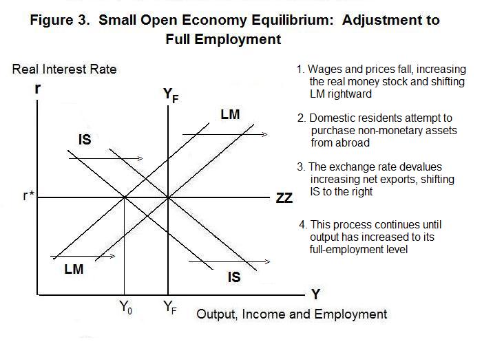
The process of adjustment to full employment is shown in Figure 3. The initial less-than-full-employment income level is Y0 . Excess supply in the labour market eventually leads to declines in wages and firms competitively pass these cost reductions on in lower prices. The real money stock M/P increases, shifting LM to the right. The resulting portfolio adjustment pressure on the exchange rate causes Π to rise, lowering Q and shifting world demand onto domestic output. This shifts IS to the right along with LM, until the two curves intersect along the ZZ line at the vertical full-employment line YF .
Time for a test. Be sure and think up your own answers before looking at the ones provided.
Question 1
Question 2
Question 3
Choose Another Topic in the Lesson.