Let us treat savings S , net investment I ,
the trade balance BT and the debt service
balance DSB as desired magnitudes, all expressed in
real terms. How then does the equality
1. S − I = BT + DSB
arise? To proceed we must analyze the factors determining the
levels of savings, investment and the balance of trade. The debt
service balance in each period is determined by previous borrowing
and lending abroad as reflected in the current state of the balance
of indebtedness.
Start with the balance of trade, which is equal to domestic exports
minus imports. Like any commodity aggregates, the desired quantities
of exports and imports will depend on incomes and relative prices.
A rise in domestic income will increase imports and, if the country is
small, reduce exports as a result of the fact that more domestic
export goods are consumed domestically instead of being sold on the
international market. The result will be a negative effect on the
balance of trade. Correspondingly, a rise in income abroad will
increase foreign imports (domestic exports) and have a positive
effect on the domestic balance of trade. Higher prices of
domestic goods in terms of foreign goods will cause both domestic
and foreign residents to substitute foreign goods for domestic
goods in their consumption and investment plans. This will cause
imports to increase and exports to decline, leading to a decline
in the balance of trade.
These principles can be expressed in terms of the following linear
equation:
2. BT = ΦBT − m Y
+ m* Y* − σ Q
where m and m* are the domestic and
foreign marginal propensities to import, Y and Y*
are domestic and foreign incomes, ΦBT is a
constant reflecting tastes and other factors that affect
exports and imports at given incomes and relative prices, and Q
is the relative price of domestic goods in terms of foreign
goods. The marginal propensity to import is the real expenditures
on net imports associated with a one-unit increase in real income. The
relative price of domestic goods in terms of foreign goods is in fact
the real exchange rate. All three parameters, m ,
m* , and σ , are positive.
The real exchange rate is defined as
3. Q = P / Π P*
where P and P* are the domestic and foreign
price levels and Π is the nominal exchange rate defined as the
domestic currency price of foreign currency. The denominator of the right
side of Equation 3 gives the foreign price level measured in domestic currency
units. Q is thus the price level of domestic goods divided by the
price level of foreign goods where both price levels are measured in the same
currency. A rise in the real exchange rate can be associated with an increase
in the domestic price level, a decline in the foreign price level, or an
increase in the international value (i.e. appreciation) of the domestic currency
represented by a fall in the price of foreign currency in terms of domestic
currency.
Turning now to the net capital outflow, or savings minus
investment, we must first note that savings is the excess of
income over consumption
4. S = Y − C
where C is the level of real consumption. Consumption is portrayed in
standard Keynesian models as positively related to income and
represented by an equation like
5. C = â + mpc Y
where â is a constant reflecting changes in tastes and other
factors that affect consumption at given levels of income
and mpc is the marginal propensity to consume---that is,
the change in real consumption associated with a one unit change in real income.
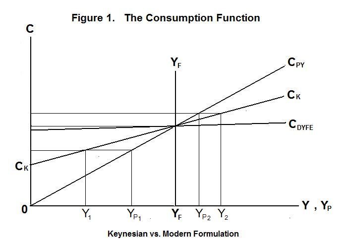
This relationship between consumption and income is shown in Figure 1. The
standard Keynesian consumption function is represented by the line
CK. The marginal propensity to consume, which is
represented by the slope of the line, takes a positive value between
zero and one. As current income, denoted by Y increases along
the horizontal axis, consumption increases less and less proportionally than
income.
We now turn to the question of how the equality of the
desired net capital outflow and the desired current account
surplus is brought about. As you should know from the previous
topic, this is the same equilibrating mechanism that brings about
equality aggregate demand and supply. Variables in the economy
must adjust to bring about equality of the relevant desired
magnitudes. We now address the question as to what these variables
are and how the adjustment process works.
Important refinements of this Keynesian view of consumption were introduced by Milton Friedman and Franco Modigliani. Friedman expanded upon the idea that consumers smooth consumption through time, basing it on their expected average level of future income, or permanent income, rather than on the current level of income. This permanent-income consumption function is denoted by the line CPY in Figure 1 with the horizontal axis now measuring the level of permanent as well as current income. Unlike the Keynesian current-income consumption function, the permanent-income consumption function passes through the origin, The reason why the current-income consumption function is flatter than the permanent-income consumption function is that consumption will be higher relative to current income when current income is below permanent income and lower relative to current income when current income is above permanent income. This can be seen from the current and permanent income levels 1 and 2 in Figure 1. The principle that consumption depends on permanent income rather than current income is necessary to avoid the concluding that rich people will necessarily get continually richer relative to poor people because as their wealth grows they will save larger and larger fractions of their income.
Modiglani's refinement was to note that the fraction of their incomes people spend on consumption depends on where they are in the life-cycle. Young people tend to consume more than their income because they are borrowing (often from relatives) to finance their education and their start in life. Then as they reach middle age these individuals consume less than their income, paying off their earlier borrowings and accumulating capital assets to support them in their old age. And in their elderly years they again consume more than their income, drawing down their capital stock to whatever level they wish to leave to their heirs. It turns out that Modigliani's life-cycle theory is fully consistent with Friedman's permanent income theory in explaining aggregate consumption when the age distribution of the population remains the same through time.
Modern theories of extended families' inter-temporal maximization of utility, where each generation receives utility from the consumption opportunities of subsequent generations, suggest a further refinement of the permanent-income-life-cycle theory. If we correctly treat expenditures on consumer durables as investment rather than consumption, which is limited to the income flow off those durables, it is reasonable to expect that consumption as narrowly defined should grow along with overall wealth at a practically constant rate. During good years, the higher levels of current income relative to consumption will be channeled into capital investment. Then in bad years that capital will be drawn down to maintain consumption in the face of current low levels of income. When full-employment income is denoted by the vertical line YF in Figure 1, the consumption function with respect to deviations of income from full employment will be much flatter than the Keynesian consumption function, with practically none of the deviations on current income around its full-employment level being consumed. This is shown by the line CDYFE in Figure 1. Keep in mind that the Keynesian consumption function relates consumption to all changes in income, whether temporary or permanent.
The above analysis noted that a considerable part of what appears as variations in consumption through time really represents variations in capital investment in consumer durables. The lower income segment of the population will find it difficult to borrow at reasonable interest rates to maintain consumption during an economic downturn. Instead, those individuals will allow their clothes, cars, refrigerators, and other durables to wear out, replacing them during the subsequent economic upturn. Of course, the depreciation of the existing stock of durables implies some reduction in the consumption of the services of those durables and the expansion in good times implies some increase in the consumption of those services. Also, we cannot rule out a tendency of people to cut some luxury pure consumption items such as travel and restaurant expenditures during adverse times and to splurge a bit in good times. Hence it is reasonable to expect some effects of deviations of income around full-employment levels on aggregate consumption. Nevertheless, it is also reasonable to assume that the bulk of deviations of income around full-employment levels will be channeled into savings.
From Equation 4 we can thus express the full-employment level of savings as
6. SF = YF − CF = YF − (YF CF / YF) = (1 − ξ) YF
where ξ is the rato of consumption to income under normal full-employment conditions. The deviation of savings from its full-employment level can be expressed as
7. S − SF = Y − YF − (C − CF) = (1 − γ) (Y − YF)
where, of course, Y − YF and C − CF are the deviations of income and consumption from their full-employment levels and γ measures the response of consumption to deviations of income from its full-employment level. To the extent that γ is small so that consumption does not deviate much from its full-employment level, most of the deviations of income will be channeled into savings. Although permanent income and full-employment income need not be the same, deviations of income around its full-employment level will surely be transitory.
The determinants of the level of real investment can also be represented by a linear relationship
8. I = δ − μ r
where r is the domestic real interest rate and δ incorporates shifts in expectations, investment opportunities, and other factors that affect investment at given real interest rates. Since the market in assets is world-wide, the domestic real interest rate is determined by conditions in the world market at the level r* which is equal to the world real interest rate plus the risk premium on domestic assets plus the expected rate of decline in the domestic real exchange rate, and represented by the line r*Z in Figure 2. Equation 8 can thus be rewritten as
9. I = δ − μ r*
where μ is positive so a rise in world interest rates has a negative effect on domestic investment.
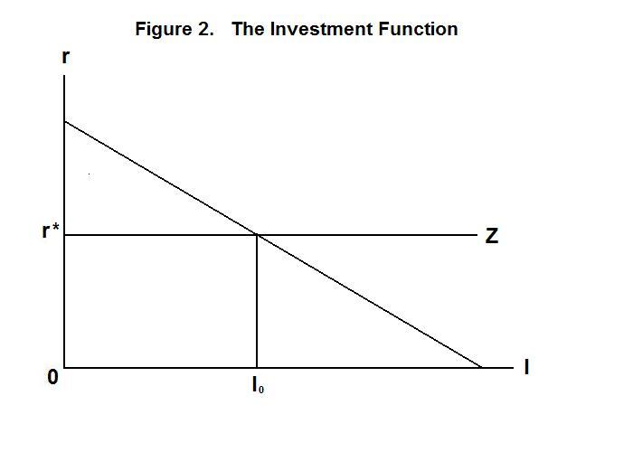
The equation determining domestic real investment, called the investment function, is shown in Figure 2. The relationship between the real interest rate and the level of investment is negatively sloped because a fall in the interest rate increases the present value of the income flows from capital, making a wider range of potential investment projects profitable. The lower the interest rate, therefore, the greater the level of real investment. One would also expect that investment would be positively associated with the level of aggregate output and income, given that higher income levels will widen the range of profitable investment projects. This effect is ignored here because it complicates things without changing any of the conclusions. Also, the assumption that the investment function is a straight line is strictly for expositional convenience---there is no basis for any particular assumption about the shape of the investment function apart from its negative slope.
The savings and investment equations and the balance of trade equation can now be substituted into Equation 1 to yield
10. ΦS-I + s Y + μ r* = ΦBT − m Y + m* Y* − σ Q + DSB
where ΦS-I represents factors affecting the excess of savings over investment other than income and the world real interest rate, ΦBT represents the factors affecting the balance of trade other than incomes and relative prices and s , the marginal propensity to save, equals (1 − ξ) when there is continuous full employment or (1 − γ) otherwise. Since Y* and r* are determined in the rest of the world, DSB is determined by previous international borrowing and lending, and ΦS-I and ΦBT are constants, the only variables that can adjust to preserve the equality in Equation 10 are the level of domestic income Y and the real exchange rate Q . Either or both of domestic income and the real exchange rate must adjust to keep the left-hand side of Equation 10 equal to the right-hand side.
If we assume full employment of the domestic economy or, alternatively, compare two points in time over which the level of domestic unemployment is the same. Then the only variable that can adjust to preserve equilibrium is the real exchange rate.
Suppose world investors come to believe that the domestic economy is a better place to invest than previously thought. This will appear as a decline in ΦS-I on the left side of the equality, so Q must increase to reduce the right side by the same amount. A shift of world investment into the domestic economy thus increases the relative price of domestic goods in terms of foreign goods. This can happen in one or both of two ways---the domestic price level can rise, or the domestic currency can appreciate in the international market. This real exchange rate adjustment occurs because the increase in investment creates upward pressure on aggregate demand, so Q must rise to reduce the pressure of net exports on aggregate demand and to accomodate the resource demands of the additional investment.
Now suppose that there is still full employment and that domestic residents' tastes change so that they choose to import more from abroad than before. The left side of Equation 10 will remain unaffected, while ΦBT will decline, reducing the right side. This decline in the right side of Equation 10 cannot take place if the economy is to remain in equilibrium, so Q must fall to increase net exports back to where they were before tastes changed. An upward shift in exports or downward shift in imports would have the opposite effect.
Now consider the case where there is less than full employment in the domestic economy. Following standard Keynesian tradition, let us assume that less than full employment is associated with a constant price level and also that the government happens to be maintaining the nominal exchange rate fixed. These assumptions imply that Q is constant, so all of the adjustment must now fall on Y . A shift of world investment into the domestic economy---that is a fall in ΦS-I must increase domestic output and income to the point where savings have increased sufficiently on the left side of Equation 10 and imports have increased sufficiently on the right side to keep the two sides equal.
And an exogenous upward shift of net exports, represented by an increase in ΦBT on the right side of Equation 10, will lead to an increase in Y until the left side has increased and the right side has declined (from its initially higher level) to preserve the equality.
It should be understood, of course, that nothing requires that all the adjustment fall on Y under less than full employment conditions. If the exchange rate is allowed to float freely, the above less-than-full-employment adjustments can fall partly on Q and partly on Y .
It is time for a test. Be sure to think up your own answers before looking at the ones provided.
Choose Another Topic in the Lesson