Let us look again at the goods and asset market equilibrium
conditions of the small open economy expressed here respectively as
Equation 1 and Equation 2
1. Y
= ( a + δ
+ ΦBT + DSB)/(s + m)
− μ/(s + m) r
+ m*/(s + m) Y*
− σ/(s + m) Q
2. r*
= − (1/θ)( M/P + ΦM )
−
τ + (ε/θ) Y
where Y and Y* denote domestic and foreign output and
income and employment, ΦBT represents exogenous
shocks to the balance of trade, DSB is the debt service balance,
Q is the real exchange rate, defined as the relative price of
domestic in terms of rest-of-world output, r* is the domestic real
interest rate which, is determined by world market conditions, s is
the domestic marginal propensity to save, m and m* are
the domestic and foreign marginal propensities to import, M is the
nominal money stock, P is the domestic price
level, ΦM represents an exogenous shift factor in
the demand for real money balances and τ is the expected rate
of domestic inflation. Tariffs and export subsidies operate by increasing
ΦBT in Equation 1, shifting the IS curve to the
right.
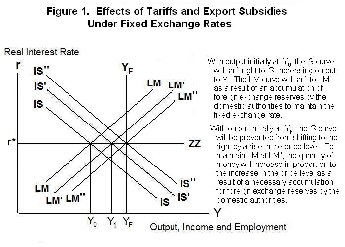
Given a fixed exchange rate and less-than-full-employment, the price level
and the nominal exchange rate and hence the real exchange rate are fixed in
Equation 1. At the given world real interest rate, this leaves only one level
of Y consistent with domestic goods market equilibrium. Equilibrium output
is determined by the intersection of the IS curve and the ZZ line in panel of
Figure 1. If there is full employment and a fixed exchange
rate the price level and the real exchange rate will adjust to force the IS
curve to pass through the ZZ line at the full-employment level of output
YF .
The money supply will adjust endogenously through changes in the stock of foreign
exchange reserves to drive the LM curve through the IS-ZZ intersection.
Alternatively, of course, the monetary authority could create the
equilibrium stock of nominal money balances by open market operations in
domestic bonds, eliminating the need for foreign exchange reserve adjustments.
By fixing the nominal exchange rate the government gives up control over the
nominal money supply---it must create the equilibrium nominal money stock by
purchasing and selling either domestic assets or foreign exchange
reserves.
A tariff, import restriction or export subsidy increases
the current account balance at each level of the real exchange
rate, shifting world demand onto domestic goods. The
IS curve shifts to the right and, given a fixed nominal exchange
rate and less-than-full employment, the equilibrium level of Y
increases from Y0 to Y1 in
Figure 1. The money supply increases automatically, driving LM to the
right until it crosses through the new IS-ZZ intersection. These policies
are effective in increasing the level of employment under fixed exchange
rates.
An alternative approach to increasing aggregate demand
for domestic goods in slack economic times is to put tariffs
and quotas on imports or to subsidize domestic exports. Such
initiatives are typically referred to as commercial policy.
Commercial policy operates by shifting world demand for
goods and services off foreign and onto domestic output.
If there is full employment, and the equilibrium is therefore at output YF in Figure 1, the price level will increase to eliminate the expansion of exports relative to imports and the rightward shift of IS, preventing output from rising above YF. The rise in P will require a proportional rise in M to keep LM from shifting to the left from the IS-ZZ-YF intersection. This increase in the money supply will occur automatically through an accumulation of foreign exchange reserves by the domestic authorities in order to maintain the fixed level of the nominal exchange rate.
Now let us assume a flexible exchange rate regime. Given a fixed price level and an exogenously determined nominal money supply in Equation 2, there is only one level of Y consistent with asset equilibrium. When this level of Y is plugged into Equation 1, there is only one level of the real (and nominal) exchange rate consistent with goods market equilibrium. The effect of the commercial policy on the IS curve will be eliminated by an appreciation of the exchange rate and output will remain at Y0 in Figure 2 where the LM curve continues to cross the ZZ line. The equilibrium level of income is determined by the intersection of LM and ZZ, with the nominal exchange rate continually adjusting to drive IS through that intersection. Were income to increase, there would be an excess demand for domestic currency on the foreign exchange market as domestic residents attempt to maintain asset equilibrium by selling assets to acquire the additional money demanded at that higher level of income.
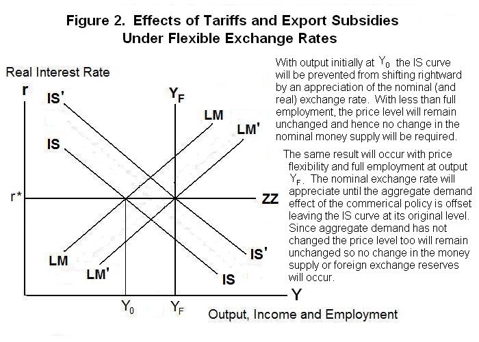
When there is full-employment the nominal exchange rate will again appreciate to prevent the IS curve from passing through the ZZ line at an output greater than YF. Since the effect of the commercial policy on aggregate demand is again offset, there will be no effect on the price level and, hence, no change in the stock of foreign exchange reserves and nominal money supply will be required to maintain the LM curve at its initial level.
Under a flexible exchange rate regime, the authorities cannot permanently shift the IS curve to the right by raising tariffs, putting quotas on imports or subsidizing exports. Any tendency of IS to shift to the right will raise income and increase the quantity of money demanded. Domestic residents will try to sell assets to foreign residents to increase their money holdings. This will cause an appreciation of the nominal (and real) exchange rate, driving IS back to its original position. These policies are thus ineffective devices for raising domestic output and employment under flexible exchange rates.
Because commercial policies of the sort discussed above increase domestic output and employment (under fixed exchange rates) by shifting world demand off foreign and onto domestic goods, they have the effect of reducing employment in the rest of the world. While this effect is of trivial magnitude when the domestic economy is very small, a simultaneous attempt on the part of all countries to increase employment by putting tariffs on imports will be ineffectual. Each country expands at others' expense, so the overall employment effects will cancel out and efficiency gains from international trade will be sacrificed. For this reason these policies are called beggar-thy-neighbor policies.
Notice that monetary policy under flexible exchange rates is also initially a beggar-thy-neighbor policy---a domestic monetary expansion causes domestic residents to try to purchase assets abroad with the excess cash, leading to a devaluation of the domestic currency and an expansion of exports relative to imports which increases the aggregate demand for domestic output at the expense of output and employment abroad. But there is an important difference between the effects of monetary policy under flexible exchange rates and those of commercial policy under fixed exchange rates. True, when all small countries expand their money supplies the effects on their trade balances will be offset by the monetary expansion in the rest of the world. But at the same time the world money supply will increase and the world interest rate will fall. As can be seen from Equation 1 above, a fall in the world interest rate will reduce the individual countries' interest rates and increase output and employment in every country. These effects will be discussed in the next lesson which deals with big-open-economy equilibrium.
Finally, we should note that fiscal policy under fixed exchange rates is not a beggar-thy-neighbor policy. A fiscal expansion in a small open economy leads to an increase in its imports and a decline in its current account balance. Other countries' current account balances must therefore increase, so domestic output expansion induces output expansion in the rest of the world---neighbors are not beggared!
Time for a test. Be sure and think up your own answers before looking at the ones provided.
Question 1
Question 2
Question 3
Choose Another Topic in the Lesson.