Consider wage determination in a typical
non-unionized industry in an economy. The analysis is conducted
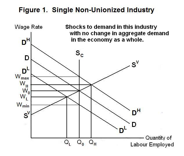
with reference to Figure 1. Suppose that the general price level
in the economy is constant but that there are period-to-period
fluctuations in the demand for the industry's output. The demand
for labour in the industry is on average at DD, but shifts up to
DH for half the time and down
to DL for the rest of the time.
These fluctuations reflect shocks to the demand for output in this
industry relative to other industries and not aggregate demand
shifts in the economy as a whole. Given the constant price level,
movements in the wage rate along the vertical axis represent real
wage changes in the industry relative to the rest of the economy.
We begin our analysis of economy-wide fluctuations in
the level of employment by making the absolute minimum departures
from the neoclassical assumptions of homogeneous workers who,
along with firms, have no individual influence on wages paid.
An auction mechanism is assumed in the background to effect an
immediate response of wages to market conditions.
We use the term cyclical unemployment to refer to movements
of employment over what is commonly called the business cycle,
as opposed to changes in the natural or frictional level of
aggregate unemployment.
The effect of the fluctuations in demand for the industry's output will depend on the supply curve of labour to the industry. If workers prefer to work a constant amount every period and let their real wage rate fluctuate between Wmin and Wmax, their supply curve will be the vertical curve SC. It is more likely, however, that they will choose to work more in boom periods, when the wage rate is high, and less in slack periods, when the wage rate is low. This employment response to the variation in the opportunity costs of working rather than taking leisure is given by the curve SVSV. The wage rate in the industry will thus be WH in good periods and WL in bad periods.
Alternatively, let us suppose that there are fluctuations in the demand for output in the industry of the same magnitude as before but that these fluctuations represent fluctuations in nominal aggregate demand and are thus common to all industries in the economy. Assume also that all workers and firms know the nature of these fluctuations, which are portrayed in Figure 2. Both workers and the firm---indeed, all workers and firms in the economy---will find it in their interest to adjust wages and prices to keep output and employment constant. There is no reason to make real output and employment adjustments to economy-wide nominal shocks. The nominal wage rate will thus fluctuate between Wmin and Wmax and the general price level will move in the same proportion with real wages remaining constant.
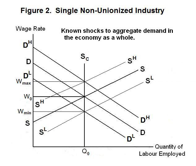
Workers shift their supply curve (which shows their response to nominal wage movements at a constant general price level) upward to SHSH and downward to SLSL to maintain their real wage rates and employment constant in the face of the rising and falling general price level as nominal aggregate demand shifts. Firms pass these nominal wage increases and decreases through to their product prices, maintaining the real prices of their outputs in terms of aggregate output constant. The situation is one of complete wage and price flexibility in response to economy-wide inflation and deflation of nominal aggregate demand.
Now, as a third option, let us suppose that workers and firms observe the nominal demand shocks but do not know whether these shocks are specific to their industry or economy-wide. When economy-wide shocks are extremely rare and specific industry shocks are frequent, it is natural for them to interpret observed nominal demand shifts as the result of local-industry shocks. In this case, the response will be the same as that in Figure 1. When the shock is positive and economy-wide, the nominal the nominal wage rate would have to rise to Wmax to maintain the real wage constant. Since it will rise only to WH, the real wage rate will fall. When the shock is negative the nominal wage rate will fall to WL and the real wage rate will rise. The level of employment changes to QH in boom periods and to QL in recessions. These employment fluctuations are involuntary in the sense that workers would have chosen to set their wages at Wmax and Wmin and keep employment constant at Q0, as in Figure 2, had they known that the shocks were economy-wide.
The aggregate unemployment rate in the economy will thus fluctuate about its natural level due to misinformation on the part of workers and firms as to the source of the shocks to demand in their individual industries. Workers and firms think the shocks are industry specific when in fact they are economy-wide.
When both industry-specific and economy-wide shocks occur frequently, workers and firms will attach some probability to an observed shock being economy-wide. The supply labour supply curve will shift upward or downward to reflect the expected shift of the price level. When the price level is expected to remain unchanged in the in the current period compared to last period, the labour supply curve will be SS in Figure 3. When the price level is expected to be higher relative to last period the supply curve will be higher by an appropriate amount, say at S+S+. When price level is expected to be lower than in the previous period, the labour supply curve will be similarly lower, say at S-S-.
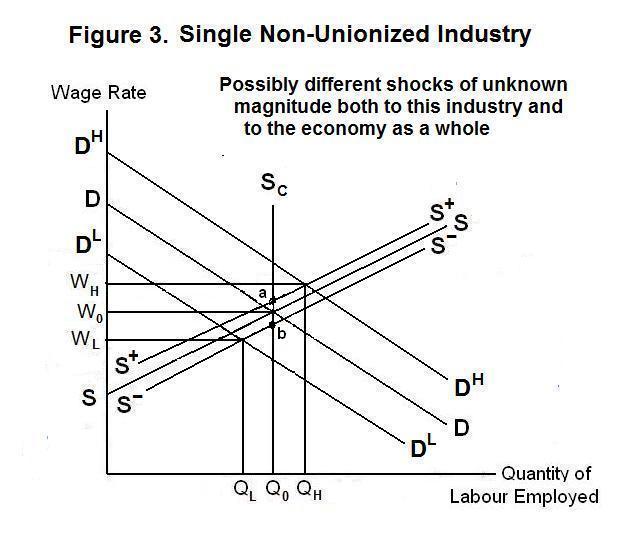
If industry-specific shocks have been frequent and economy-wide shocks infrequent in the past, workers and firms will attach a small probability to an observed shock being economy wide. The labour supply curves will shift by small amounts in response to observed shocks as shown in Figure 3, and the fluctuations in employment around its natural level in response to economy-wide shocks will be substantial. If economy-wide shocks have been frequent in comparison to industry-specific shocks in the past, workers and firms will attach a high probability to a given shock being economy-wide. The labour supply curves will shift by a large amount and the fluctuations in employment about its natural level will be small as shown in Figure 4. In both Figure 3 and Figure 4, the points a and b on the ScQ0 line represent the nominal wage rates at which the real wage rate is expected to be constant---if the estimations of the shifts in aggregate demands were correct, the DH and DL lines would have passed through these respective points. The vertical distance of point a from the horizontal axis gives the nominal wage rate that will maintain the real wage rate constant in the face of the expected increase in aggregate demand so the distance between the W0Q0 intersection and point a gives the increase in the price level that was expected. Similarly, the distance between the W0Q0 intersection and b gives the expected fall in the price level in the case of the decline in aggregate demand so that the distance between b and the quantity axis is the nominal wage rate expected to maintain the real wage rate constant in that case.
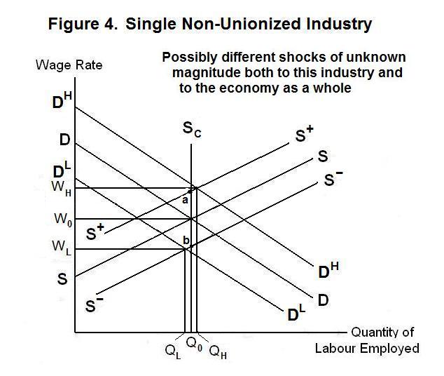
Higher wages will necessarily get passed on to higher prices. Thus, when aggregate demand is unexpectedly high and actual wages rise relative to expected wages ( WH > a Q0 ) the actual price level will rise relative to its expected price level. And when aggregate demand is unexpectedly low ( WL < b Q0 ) the actual price level will fall below its expected price level. Furthermore, it is clear from the two figures that when the actual price level increases relative to the expected price level employment increases above its natural level, and when the actual price level declines relative to the expected price level the level of employment falls below its natural level.
Given that aggregate output will rise above its natural or long-run equilibrium level when aggregate employment rises above its natural level, and fall below its natural level when employment falls below its natural level, we can express aggregate supply as
where Yf is the natural or full-employment level of output, PE is the expected price level and β > 0. This equation is called the Lucas-Supply Curve after its inventor, the Nobel-Prize-winning economist Robert E. Lucas (1938- ).
When workers' and firms' expectations about the equilibrium price level are correct, and P = PE , aggregate employment and output will be at their natural or full-employment levels. When aggregate demand expands beyond where workers and firms think it will expand the actual price level will rise above the expected price level and aggregate output and employment will expand above their full-employment levels. And when aggregate demand contracts relative to what workers and firms expect, the actual price level will be below the expected price level and output and employment will fall below their natural or full-employment levels.
We thus arrive at a theory explaining fluctuations of aggregate output and employment about their natural or full-employment levels. Less-than-full-employment arises when aggregate demand unexpectedly falls, resulting in declines in the level of nominal wages. Because they do not realize that aggregate demand has fallen, workers think that real wages in their industries have fallen below normal levels and mistakenly substitute leisure for work, moving to the left along what turns out to be the wrong supply curve of labour. In periods of expansion, the opposite happens. Workers fail to realize that aggregate demand has expanded and think that the observed increase in their wage rates represents a rise in real wages resulting from a temporary positive shock to the demand for output in their industry. They then substitute work for leisure in response to what they think are temporarily high wage rates. Workers should shift their supply curves up and down with the fluctuations in aggregate demand but fail to fully realize the extent of changes in aggregate demand, thinking that the demand for output in their industry is shifting. Movements of nominal wages are then partly mistaken for movements in real wages, bringing about substitutions between work and leisure in response to perceived changes in opportunity costs.
This is an interesting theory of unemployment in that it shows how far we can get by dropping only one assumption of traditional neo-classical economics---the assumption that everyone has perfect information. Nevertheless, the theory is quite unsatisfactory as a proposed explanation of unemployment during the Great Depression of the 1930s. It would have us believe that 20 percent of the labour force was unemployed during these years because workers mistakenly decided to take time off, thinking that real wages were below normal levels. In fact, people desperately wanted jobs at prevailing wages but no firms would employ them!
There is an interpretation of the auction theory that makes sense in terms of explaining cyclical movements of the level of employment in the absence of changes in the unemployment rate as usually defined. Workers may indeed work more overtime or postpone holidays and thereby contribute more labour in periods in which they think that the real wage rate is above its normal level and take less overtime and more holidays, and non-paid leave, when they think that the real wage rate is below its normal level. But these changes in employment, while they may be cyclical, must be interpreted as voluntary. As an explanation of involuntary unemployment, where people want jobs but cannot find them, this auction theory is totally unsatisfactory. It implies that workers tend to quit their jobs to take leisure in recessions and hang on to their jobs in boom periods to work harder. On the contrary, the empirical evidence suggests the opposite: that workers tend to quit jobs for better opportunities in good times and desperately hang on to their jobs in bad times. Moreover, firms tend to lay off workers in bad times and hire extra workers in good times. The auction theory provides no explanation of this tendency of firms to lay off workers in periods of recession. So we need to pursue additional avenues of analysis to explain why unemployment occurs.
But first, a test! Think up your own answers before looking at the ones provided.
Question 1
Question 2
Question 3
Choose Another Topic in the Lesson