The net benefit to consumers from consuming a product is
equal to the area under the demand curve up to the quantity consumed
minus the amount the consumer has to pay to purchase that quantity.
This payment is received by the producers of the commodity.
It can be divided, depending on the situation, into an
opportunity cost portion and a rent portion. The rent portion
is often called producer surplus. It is the excess of
the total payment to producers over and above what would be required to
get them to produce the quantity of the good consumed. This contrasts
with the consumer rent or surplus which is the total benefit received by consumers
over and above what they have to pay to purchase the quantity of the
good consumed.
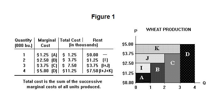
Let us use Figure 1 to analyze the production of an agricultural
product---say, wheat---in a local area. Suppose that the
farmers in the area have available to them a fixed stock of land
but can hire all the labor and capital they want at fixed wages
and machine rental prices. As more and more labor and capital
inputs are applied to the fixed stock of land, the additional
increments of output that can be obtained with successive applications
of additional labor and capital get smaller and smaller---that
is, there are diminishing returns from the application of
labor and capital on land.
Suppose that $1250.00 of labor and capital resources have to be used to produce the first thousand bushels of wheat. This means that farmers will have to obtain $1.25 per bushel to make it worthwhile for them to produce these thousand bushels. Let us further suppose that, due diminishing returns, it takes $2500.00 worth of labor and capital to produce the second thousand bushels of wheat. Farmers will have to receive $2.50 per bushel to get them to produce this additional output.
It turns out, however, that when the price of wheat is $2.50 per bushel, as is required to get farmers to produce 2000 bushels, they receive $2.50 per bushel for all the wheat they produce, not just for the last thousand bushels. Farmers thus pay $1250.00 + $2500.00 = $3750.00, represented by area A plus the area B in Figure 1 for the labor and capital resources (including, of course, appropriate payments to themselves for any of their own labor they use) to produce the 2000 bushels of wheat, and are then able to sell this wheat to consumers for $2.50 × 2000 = $5000.00, represented by area A plus area B plus area I in Figure 1. They earn a surplus, or rent, equal to $1250.00 represented by area I. This can be thought of as a rent to land. If someone other than the farmer owned the land she could charge the farmer $1250.00 for the use of it and the farmer would still find it worthwhile (barely) to produce the 2000 bushels of wheat.
Even though someone has legal title to the land and can charge for its use, the land is really free from the point of view of society as a whole. It is what one of the founders of modern economics, David Ricardo (1766-1823), called "the natural and indestructible powers of the soil", freely available to man without any required expenditure of resources. This contrasts with tractors, cultivators and trucks, which have to be produced using labor and capital that could otherwise be used to produce something else. Land is thus available to society at zero alternative opportunity cost. Even if the government were to tax away all the economic rent to it (the $1250.00 in the above example) the land would continue to be fully used in production.
The economic rent to land can also be shown on a graphical representation of the supply and demand for land. The supply of land is the vertical line S in Figure 2, where the stock of land available for wheat production is aggregated into a single unit. The demand curve for land is negatively sloped because an expansion of the quantity of land would mean that less labor and capital would have to be used per unit of land in producing each each level of output. The pressure of diminishing returns will therefore be lower and the rent to land will be less.
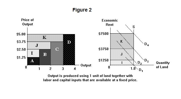
When 1000 bushels of wheat are being produced the demand curve for land, D1, crosses the supply curve at a zero rent to land. As output increases to 2000, 3000 and 4000 bushels, the demand curve shifts upward, intersecting the supply curve at $1250, $3750, and $7500 respectively. The areas I, J, and K in the right panel of Figure 2 correspond to the similarly labelled areas in the left panel.
Three general conclusions emerge which are summarized in Figure 3.
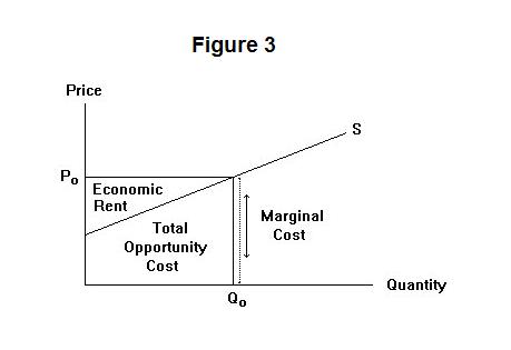
1. The marginal opportunity cost of adding a unit to quantity is the vertical distance between the supply curve and the horizontal axis.
2. The total alternative opportunity cost, which is the sum of the marginal costs, is the area under the supply curve up to the quantity supplied.
3. The economic rent is the area over the supply curve and under price received by the seller.
Notice here that rent will occur for any input whose supply
curve is upward sloping. The the rent that appears on the
supply and demand diagram for the final product is the sum of
the rents that appear on the supply and demand diagrams for the
individual inputs. This is illustrated in Figure 2, where the areas
I, J, and K are
each of identical size in the left and right panels. In this case
only one input, land, receives rent while the other inputs,
labor and capital, have perfectly elastic supply curves and
receive no rent.
The prime example of rent to labor is the situation faced by star professional athletes. The demand and supply situation for the hockey services of a superstar like Wayne Gretsky is illustrated in Figure 4. Assume for the sake of discussion that Wayne could have earned $50,000 per year in his next best occupation---say, sales---if he could not play hockey. Suppose also that he liked playing hockey so much that he would have actually be willing to play for, say, $30,000 per year. Since he was so talented, the demand for Wayne's hockey-playing services by the public, taking into account the costs of running the team and paying all other expenses, was $5,000,000. The supply curve for Gretsky's hockey services is the L-shaped curve SS and the demand curve for his services on the part of the public is DpDp.
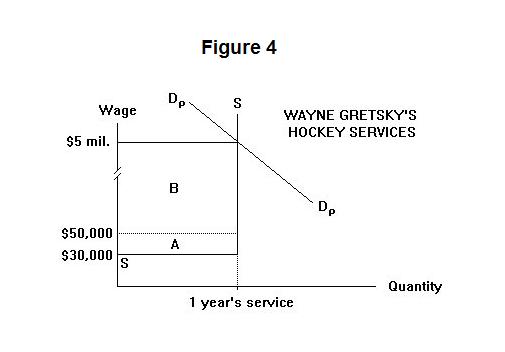
Now what would Wayne Gretsky actually be paid? This depends on the legal arrangements under which he was allowed to sell his services. If all hockey players were free agents and could thus sell their services to the highest bidder, the market price for Wayne Gretsky would be $5 million per year. His opportunity cost would be $30,000 and the difference is economic rent. Note that the rent is divided into two parts, the difference between what Wayne was worth to society playing hockey and what he could earn in his next best occupation---area B ---and the surplus that Wayne himself got from the fun of playing hockey rather than doing something else, represented by the area A.
In earlier days each hockey player was assigned as a teenager to the team having exclusive rights to players in his geographical area, and from that point on was "owned" by that team. Under these circumstances the team could pay Wayne Gretsky $30,000 since he had no other opportunity to sell his hockey services and loves playing hockey---the rent from Wayne's hockey-playing services would thus captured by the owner of the team. Actually, the team would pay Gretsky more than $30,000, though far less than $5 million, both to encourage both him and other players to play their best, and to avoid the embarrassment of seeming to exploit him.
In modern times players in most professional team-sports are owned by their current teams but have certain rights to free agency. These rights are enforced by contracts between the league and the players' union. The players' economic rents are thereby divided between themselves and their team owners. In essence, the baseball and hockey strikes of 1994 were squabbles over these economic rents.
It is now test-time. Be sure to think about your answers carefully before looking at the ones provided.
Question 1
Question 2
Question 3
Choose Another Topic in the Lesson.