As we noted in concluding the last Topic, the manipulation of domestic interest
rates in accordance with a Taylor Rule makes no sense for small open economies
and monetary policy in those countries operates through its effects on nominal
and real exchange rates.
One option for small countries is to fix the domestic exchange rate with respect
to a large country like the United States and then free ride off that country's
monetary policy---there is no reason to expect that those running monetary
policy in the United States, for example, would on average do better or worse than
those in charge of domestic monetary policy. This is not a good option, however,
unless there is complete freedom of migration of labour between the domestic economy
and the country whose currency the domestic currency is being pegged to. Recall
that the real exchange rate is equal to
Q = Π Pd / Pf
where Q is the real exchange rate, Π is the nominal
exchange rate, here defined as the foreign currency price of domestic currency, and
Pd and Pf are the domestic and
foreign price levels. Since this equation can be equivalently written as
Pd = Q Π Pf
it is clear that fixing the nominal exchange rate imposes a requirement that the
domestic price level vary in proportion to movements in the real exchange
rate in addition, of course, to movements in the price level abroad. This would
pose no problem if purchasing power parity holds, and the real exchange rate is
therefore constant. But purchasing power parity clearly does not hold, as can be
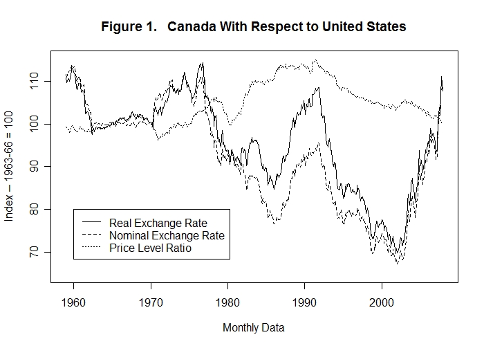
seen in the following three figures which plot the real exchange rates with respect
to the United States, along with the nominal exchange rates and price level ratios,
of Canada, the United Kingdom and Japan.
Notice first that the real and nominal exchange rates tend to vary together and that the ratios of the Canadian, British and Japanese price levels to the U.S. price level vary much more smoothly than the exchange rates.
Had Canada maintained her exchange rate with respect to the U.S. dollar fixed after 1970, the Canadian price level would have had to rise by about 10 percent relative to the U.S. price level during the 1970s, then fall by more than 20 percent between the late 1970s and 1985, then rise about 20 percent to the early 1990's, then fall by around 30 percent by 2002 and then rise by about the same amount after that year. Given the tendency of prices to be sticky in the short run, major variations in the levels of output and employment would probably have occurred. And even if output and employment were not affected the price level movements would themselves have been unacceptable. Indeed, Canada abandoned the fixed exchange rate in 1970 as a result of upward pressure on domestic prices resulting from increases in the real exchange rate.
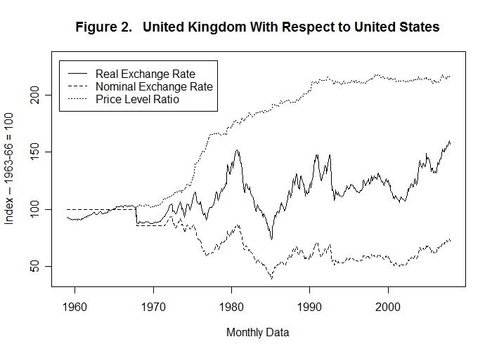
The British real exchange rate seems smoother than the Canadian one but that is an illusion resulting from the differences in the scaling of the y-axes. Had the U.K. maintained her exchange rate with respect to the U.S. dollar fixed after 1973, the British price level would have had to increase by 50 percent relative to the U.S. price level between the late 1970s and the early 1980s and fall by the same amount between the early and mid-1980s. Another 50 percent increase in the British relative to the U.S. price level would have occurred by the early 1990s followed by a sharp drop. And there would have been 50 percent increase in the U.K. relative to U.S. price level after 2002.
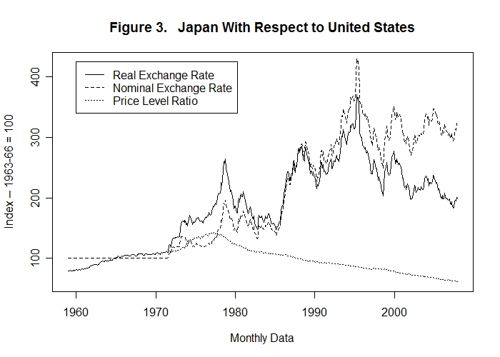
The effects in Japan would have been even more extreme. Under a fixed exchange rate the Japanese price level would have had to increase by 150 percent in the 1970s and then fall by about 60 percent by 1985. It would then have had to increase by 130 percent by the mid-1990s and then fall by nearly 50 percent by the end of the first decade of the 21st century.
These data raise an obvious question. What is causing these real exchange rate movements? As we noted in the computer-assisted learning module Small Open Economy Equilibrium V: Additional Policy Issues, a major factor might be shifts of world real capital investment towards and then away from particular countries as world technology grows. A shift of capital into a country results in an increased demand for those resources that are not internationally mobile, causing the prices of the non-traded components of domestic output to increase relative to the non-traded components of U.S. output. This will cause the domestic real exchange rate to increase, given similar prices of the traded components of domestic output at home and abroad.
Also, it is reasonable to expect that, although the traded components of each individual good will have the same price in all countries, the prices of particular traded goods in which an individual country specializes may rise relative to the prices of those traded goods it produces little of. We would thus expect that if the terms of trade of a particular country with respect to the rest of the world increases relative to the U.S. terms of trade with respect to the rest of the world, the country's real exchange rate with respect to the U.S. dollar should rise. More specifically, a rise in oil prices or commodity prices should lead to an increase in the real exchange rate of a country like Canada that specializes in producing these products.
Then there is the effect of economic growth on real exchange rates noted by Bela Balassa (1928-1991) and Paul A. Samuelson (1915-2009). As countries grow, so does the skill level of their population. And human efforts are at the core of the non-traded component of output with the result that the price of the non-traded output component, and hence the real exchange rate, should be higher in high-income countries than low-income countries. Not surprisingly, for example, the price of haircuts is many times higher in the United States than in India.
Finally, since governments tend to be forced by domestic political interests to channel their purchases of goods and services towards domestic rather than foreign production it would seem reasonable to expect that the bigger the ratio of government expenditure to income in a in a country as compared to the United States, the higher should be that country's prices of non-traded output components compared to the U.S.
The above arguments are developed much more fully in my recent book, Interest Rates, Exchange Rates and World Monetary Policy, which is published by Springer-Verlag in Heidelberg Germany. Drawing on the analysis of Part II in that book, it is useful to examine the relationship beween the Canadian and Japanese real exchange rates with respect to the United States and the factors noted above. The following table presents an ordinary least squares regression of Canada's real exchange rate with respect to the U.S. on the three of the above factors that I found significantly affected it. The prices of energy and commodities excluding energy are U.S. dollar prices, obtained from the Bank of Canada web-site, relative to the prices of U.S. exports and imports obtained from the International Monetary Fund. Logarithms of these variables and the real exchange rate are used because they best reflect the underlying relationships between the variables.
| Coefficient | Std. Error | P-Value | |
| Constant | 2.61231 | 0.29688 | < 0.00001 |
| Logarithm of Commodity Prices Excluding Energy | 0.30972 | 0.06487 | < 0.00001 |
| Logarithm of Energy Prices | 0.15435 | 0.03373 | 0.00001 |
| Net Capital Inflows / GDP: Canada minus U.S. | 0.02804 | 0.00416 | < 0.00001 |
| R-Squared = 0.77002 | |||
The signs of the variables are what one would expect and the P-Values of .00001 or less indicate that the magnitudes of the coefficients observed would occur solely on the basis of pure chance no more than once in ten thousand times. And the R-squared coefficient indicates that the variables included explain about 77 percent of the variation in the real exchange rate. Figure 4 below plots the logarithm of the Canadian real exchange rate along with the movements in it due to changes in net capital inflows into Canada as a fraction of Canadian GDP minus net capital inflows into the United States as a fraction of U.S. GDP. And Figure 5 plots the logarithm of Canada's real exchange rate with respect to the U.S. together with the movements in that real exchange rate consequent on movements in the logarithm of real energy prices.
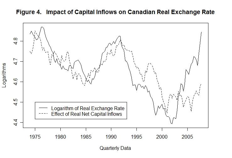
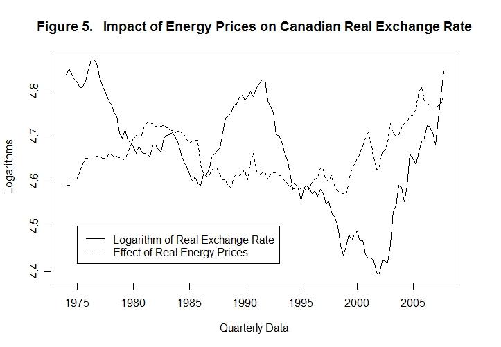
It appears that shifts in international capital movements had a major effect on Canadian real exchange rate prior to the year 2000 and that a rise in energy prices was a very important factor causing the increase in the real exchange rate after that year.
The results of an ordinary least squares regression of the logarithm of Japan's real exchange rate with respect to the United States on the factors that appear to have significantly affected it are presented in the following table.
| Coefficient | Std. Error | P-Value | |
| Constant | -9.6094 | 1.44243 | < 0.00001 |
| Logarithm of Oil Prices | 0.15997 | 0.05098 | 0.00211 |
| Gov't Consumption Expenditures / GDP: Japan minus U.S. | 0.03276 | 0.01026 | < 0.00176 |
| Net Capital Inflows / GDP: Japan minus U.S. | -0.0139 | 0.00553 | 0.01324 |
| Logarithm of Terms of Trade Ratio: Japan / U.S. | 1.23685 | 0.18818 | < 0.00001 |
| Logarithm of Japanese Real GDP | 1.22369 | 0.18182 | < 0.00001 |
| Logarithm of U.S. Real GDP | -0.8675 | 0.19114 | 0.00001 |
| R-Squared = 0.82127 | |||
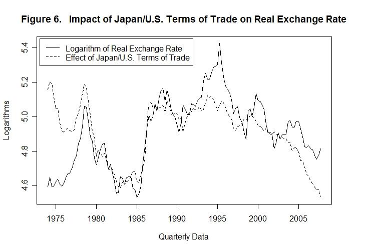
While a greater number of factors had a significant effect on Japan's real exchange rate than Canada's, only one of these had a clear graphically observable impact. Figure 6 plots the logarithm of Japan's real exchange rate together with the movements in it that resulted from changes in the logarithm of the ratio of Japan's terms of trade with respect to the rest of the world over the United States terms of trade with respect to the rest of the world. Although not shown here, it turns out that the logarithm of the terms of trade ratio was a similarly important determinant of the real exchange rates of the United Kingdom, France and Germany with respect to the United States. You should notice in the table above that Japanese real GDP was positively related to the real exchange rate and U.S. real GDP was negatively related, as predicted by Balassa and Samuelson. Statistically significant relationships between the Canadian and U.S. real GDP variables and the corresponding real exchange rate were not observable, probably because the real GDP's of Canada and the United States moved so closely together that it is impossible to distinguish their separate effects.
Is it possible that a significant part of the observed movements in the real and nominal
exchange rates were caused by the overshooting effects of monetary shocks? Recall our
analysis of exchange rate overshooting in the module Small Open Economy
Equilibrium V: Additional Policy Issues. It was there noted that overshooting
will arise when the balance of trade is slower to adjust in response to real exchange
rate shocks than asset markets adjust to portfolio shocks. Asset market equilibrium is
described by the domestic demand function for money together with an equation that determines
the level of the domestic interest rate by conditions in world asset markets and by the
expected rate of domestic inflation relative to expected inflation rates abroad. The
demand for nominal money balances can be expressed as
M = P [ ΦM − θ (r* + τ ) + ε Y ]
where θ is the absolute value of the negative interest semi-elasticity of demand and ε is the positive income elasticity of demand for real money balances. M , P , and Y , are the nominal money stock, the price level and the level of real income, r* is the level of the domestic real interest rate determined by world market conditions, τ is the expected level of domestic inflation and ΦM is a shift variable that incorporates exogenous changes in the quantity of real money balances demanded. Suppose that there is a positive shock to the nominal money stock M or a negative shock to the demand for money, represented by a decrease in ΦM , making the left side of the above equation bigger than the right side. As domestic residents re-balance their portfolios by purchasing non-monetary assets in exchange for money, the real interest rate will fall in an open economy comprising virtually the whole world until domestic residents become willing to hold the existing stock of nominal money balances. In a small open economy, where real interest rates are determined by conditions abroad, the attempt of domestic residents to purchase non-monetary assets will create an excess demand for the domestic currency in the world market leading to a devaluation. Equilibrium will be re-established when the devaluation has shifted world demand onto domestic goods to sufficiently increase the level of output and employment Y , and as a result the quantity of money demanded, under the usual assumption that the price level will not change in the short run.
The problem, of course, is that it will take some time for exports and imports to respond to movements in the nominal and real exchange rate. In the absence of some mechanism of short-run adjustment, equilibrium cannot be established. There are two possible adjustment mechanisms. First, it will normally be the case that a devaluation of the exchange rate will produce some increase in the price level P even if output prices of the goods involved are fixed---it will raise the domestic prices of the traded component of output even though the foreign prices are unchanged. The rise in the domestic price level will increase the right side of the equation to restore equilibrium. Since traded component prices represent only a fraction of domestic output, the exchange rate will have to fall much below its long-run equilibrium level to create the appropriate increase in the price level---hence the term "overshooting". This adjustment mechanism depends critically on the assumption that there is not "pricing to market"---that is, that domestic firms do not hold the prices of traded goods constant in the face of the exchange rate devaluation. A second adjustment mechanism will arise if market participants recognize that the devaluation of the real exchange rate resulting from the rise in the domestic currency price of foreign currency will eventually reverse itself. In the long run, the price level will rise in proportion to the increase in the excess supply of nominal money balances and the nominal exchange rate will devalue by the same proportion, returning the real exchange rate to its original level. Once asset holders realize that the real exchange rate is below its long-run equilibrium level and will subsequently increase they can expect a capital gain on their holdings of domestic real assets. As a result, they will bid those asset prices up and the real interest rate down. This will increase the right side of the equation until equilibrium is re-established. The problem with this avenue of adjustment is that empirical studies have established that observed real exchange rate movements tend to be unpredictable---the change between the current and next period is just as likely to be negative as positive. Of course, this empirical evidence may be simply telling us that overshooting movements of real exchange rates have not been occurring. Indeed, the table that follows shows what happens when we add unanticipated Canadian and United States base money supply shocks to the above Canadian ordinary least squares regression. Unanticipated base money supply shocks were calculated by forecasting the base money stocks in each period using an OLS regression of the stock in that period on those lags of the country's money stock and nominal GDP during the previous eight quarters that were statistically significant, and taking the percentage excess of the actual over the forecasted value as the measure of the unanticipated shock.
| Coefficient | Std. Error | P-Value | |
| Constant | 2.55168 | 0.28651 | < 0.00001 |
| Logarithm of Commodity Prices Excluding Energy | 0.32192 | 0.06363 | < 0.00001 |
| Logarithm of Energy Prices | 0.15467 | 0.03243 | < 0.00001 |
| Net Capital Inflows / GDP: Canada minus U.S. | 0.02755 | 0.00408 | < 0.00001 |
| Unanticipated Canadian Base Money Shock | 0.00497 | 0.00323 | 0.12565 |
| Unanticipated U.S. Base Money Shock | 0.00339 | 0.00516 | 0.51221 |
| R-Squared = 0.77914 | |||
Clearly, the unanticipated money supply shock variables are not statistically significant---the probabilities of the observed quantitative effects occurring on the basis of pure random chance when there are no actual effects is 12 percent in the case of the Canadian unanticipated base money shock and 51 percent in the case of the U.S. shock. Moreover, the Canadian shock has the wrong sign---a positive domestic base money shock should cause the real exchange rate to depreciate while the positive sign indicates an appreciation. Figure 7 below plots the logarithm of the actual real exchange rate along with the level of that real exchange rate after the observed effect of the unanticipated Canadian base money shock has been removed.
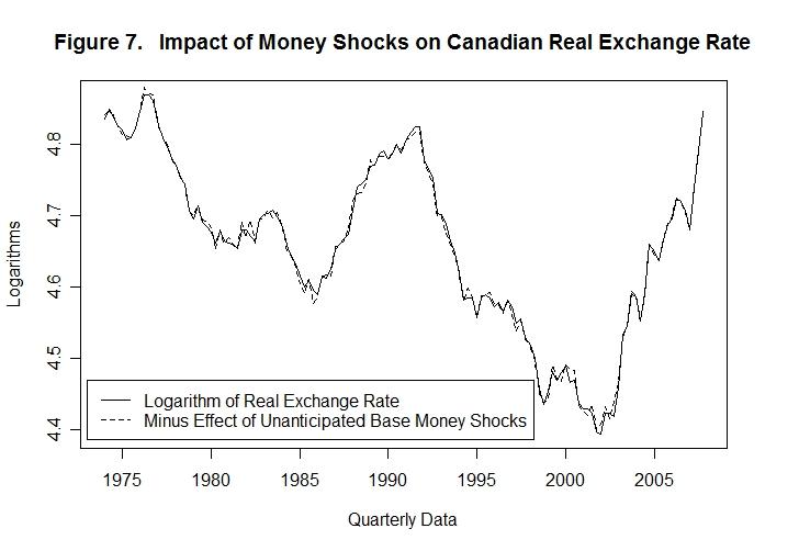
Quite apart from the fact that the sign is wrong, the observed effect is virtually zero.
It turns out that when five different methods of calculating unanticipated shocks are used, as is done in my book noted above, there is no basis for concluding that unanticipated money supply shocks have had any significant effects on the real exchange rates of Canada, Japan, the United Kingdom, France and Germany with respect to the United States.
It is obvious from the evidence presented above that flexibility of the nominal exchange rate neutralizes what would otherwise be very substantial effects of shocks to the real exchange rate on domestic output, employment and prices. This provides a strong case for flexible as opposed to fixed exchange rates when labour cannot, or will not, freely move between countries in response to real wage differences.
But flexibility of exchange rates also poses a problem. How should small countries conduct monetary policy under flexible exchange rates to avoid overshooting? Will a constant rate of money growth do the trick? If not, keeping in mind the fact that domestic real interest rates are determined in the international market, should monetary policy be conducted by raising and lowering the nominal exchange rate? Once the authorities take control over the nominal exchange rate, its equilibrium level becomes no longer observable---determining the magnitude of a policy action requires a comparison of the currently observed controlled exchange rate level with the no longer observable underlying equilibrium level.
What about a policy of maintaining a constant rate of growth of base money, or some other monetary aggregate, consistent with the underlying desired domestic inflation rate? The problem with this approach is that short-run period-to-period changes in the demand for that monetary aggregate will be transmitted into overshooting nominal exchange rate changes. It is questionable whether a constant money growth rule will work even for a big country like the United States because the demands for the individual aggregates may not move in the same direction and fluctuations of the demand for base money, or the targeted aggregate, will result in major interest rate variations. And it turns out that for a small country like Canada the variations in the demand for money are likely to be much larger than the variations in the demand for money in a big country like the United States. Indeed, as shown in my book, the variability of all Canadian monetary aggregates was much greater than the variability of the corresponding aggregates in the United States during the fixed exchange rate period from late-1962 until early-1970 when the Bank of Canada, in order to maintain the fixed exchange rate, was forced to supply whatever quantity of liquidity Canadians desired. One reason for this is that for small countries there is what might be called a "pooling advantage" of fixed exchange rates. The demand for money shocks of the many areas that form a big country like the United States are pooled into a larger aggregate that will be much less variable than the individual-area shocks as long as those individual-area shocks are not highly correlated with each other. Therefore, by fixing the Canadian dollar to the U.S. dollar, the Canadians can pool their liquidity shocks with the U.S. shocks and can therefore reduce the domestic effects on output and employment to equal the average effects over a larger area. Adopting a constant rate of money growth clearly makes even less sense for a small open economy than for a big one like the United States. The basic monetary policy objective of small countries must therefore be to obtain the "insulation advantage" of flexible exchange rates against asymmetric real shocks and, at the same time, the "pooling advantage" of fixed exchange rates against asymmetric monetary shocks.
As I noted in my book, one way for a small country's authorities to accomplish would be to maintain the nominal exchange rate movements within a narrow band for a month, then observe the real exchange rate movement that occurs over that period and adjust the range within which the nominal exchange rate will be maintained during the next period to incorporate that observed real exchange rate movement. Hopefully that would lead to a neutralization of the effects of monetary shocks together with an ultimate adjustment of the real exchange rate to neutralize the effects on it of real shocks. The problem with this approach is that the observed movements in the domestic and foreign price levels, which are necessary to calculate the equilibrium real exchange rate, will not be very accurate over periods as short as one month. And the movement in the domestic price level, and therefore the observed movement in the real exchange rate, will be much smaller than the movement in the equilibrium real exchange rate because any change in the equilibrium real exchange rate over such a short period in the face of a fixed nominal exchange rate will be transmitted into changes in output and employment rather than prices. The observed movement in the real exchange rate will therefore not reflect the underlying movement in the equilibrium real exchange rate that the authorities are trying to compensate for by adjusting the range with in which they are maintaining the nominal exchange rate.
Another option would be to intervene continuously in the foreign exchange market to eliminate any large movements in either direction, thereby removing any overshooting effect of changes in the domestic demand for money. As long as the permissible period-to-period variations in the nominal exchange rate are sufficient to incorporate the underlying real exchange rate changes, the effects of period to period shocks in the demand for money will be reduced to a noise factor. The problem, of course, is to make sure that the range of allowed variations in the nominal exchange rate is big enough to ensure that permanent movements in the real exchange rate are not being transmitted into underlying output, employment and price level changes.
A better option becomes available when we recognize that the underlying objective is to finance all period-to-period changes in the quantity of base money demanded at market participant's current expected inflation rate. In the computer-assisted learning module entitled Small Open Economy Equilibrium III: Monetary Policy under Fixed Exchange Rates, it was noted that the stock of base money equals currency plus bank reserves,
H = C + R
and the money stock equals currency plus deposits.
M = C + D
where H is the stock of base money, M is the stock of money, C is the stock of currency, R is the stock of bank reserves and D is the stock of bank deposits. Dividing the second of these equations by the first and denoting the currency/deposit ratio by c and the reserve/deposit ratio by f we obtained an expression for the money multiplier.
M/H = (C/D + 1) / (C/D + R/D) = (c + 1) / (c + f)
Given the public's desired money holdings, which we can denote by Md , and the desired currency and reserve to deposit ratios, the demand for base money can be expressed as
Hd = Md (c + f) / (c + 1)
The trick is for the authorities to continually adjust H in response to the changes in Hd , c and f that result from short-run developments and long-run economic growth to thereby maintain the rate of price-level growth equal to an inflation rate target, to which public's expected inflation rate should eventually conform. One way to do this would be to continually adjust the stock of base money to maintain the interest rate at which banks borrow reserves from each other at an appropriate level in relation to to other short-run interest rates in the economy. As Md , c and f rise and fall, the banks will put pressure on this reserve-borrowing-rate which the authorities can alleviate by providing additional, or mopping up excess, reserves to thereby move H to the level desired by the private sector. When the expected inflation rate is at its target level, this process by which H is adjusted will be pretty much automatic. Upward pressure on the desired monetary base to finance the expected inflation rate will cause the authorities to prevent an increase in the inter-bank reserve-borrowing rate by appropriately adjusting the stock of reserves. Day-to-day random fluctuations in the demand for money will also lead to upward and downward pressures on this borrowing rate which the authorities will automatically alleviate by adjustment of the reserve stock.
The problem, of course, is to choose the correct level at which to peg the inter-bank reserve borrowing rate. Pegging it at too high a level will result in banks selling other short-term assets in order to accumulate cash reserves with the result being upward pressure on the real and nominal exchange rates, while pegging the inter-bank borrowing rate at too low a level will result in accumulations of reserves by the banks that will then be indirectly used to purchase other short-term assets, putting downward pressure on the real and nominal exchange rates. Under normal conditions, the authorities will keep adjusting their target inter-bank borrowing rate so as to maintain a rate of base money growth that will finance the public's current expected inflation rate, assuming that inflation rate is also satisfactory from the central bank's point of view. During periods when the economy is weak the authorities can expand the demand for, and hence supply, of base money by lowering the inter-bank borrowing rate and in good times they can reduce base money growth by increasing that rate. When these target rate movements are of sufficient size in relation to the underlying equilibrium rate, appropriate pressures on the real and nominal exchange rates will occur---by keeping the target-rate movements sufficiently small, the authorities can ensure that resulting exchange rate changes occur very gradually and that overshooting will not occur, using open market operations to offset any excess exchange rate pressures. And excess inflationary pressures can also be handled by increasing the target inter-bank borrowing rate. An important objective of all target-rate adjustments and policy announcements, of course, is to appropriately change the public's inflation expectations---once those expectations are a the desired level, the resulting appropriate rate of base money growth will occur almost automatically. All that should be necessary to prevent overshooting is an immediate response by the authorities to day-to-day pressures on the exchange rate by accommodation of the required expansion or contraction of bank reserves.
In fact, based on calculations of the sort discussed with reference to the ordinary least squares regression results reported in the third of the three tables above, considerable unanticipated variation in the stocks of base money of the United States, Canada, Japan, the United Kingdom, France and Germany have occurred. The standard deviations of these quarterly unanticipated base money shocks are
| United States | Canada | Japan | United Kingdom | France | Germany |
| 0.97 | 1.35 | 8.46 | 1.33 | 1.88 | 0.87 |
measured as percentages. The fact that no statistically significant effects of changes in base money of these magnitudes on observed real exchange rates are observed suggests that the central banks of Canada, the U.K., Japan, France and Germany have been neutralizing the effects of unanticipated demand for base money shocks by appropriately adjusting the domestic stocks of base money. Exactly how they implemented such "orderly markets" policies can only be understood through future investigation. The potential methods outlined above are only suggestive.
Nevertheless, despite the absence of effects of unanticipated money shocks, significant changes in these countries' price levels relative to the U.S. price level did in fact occur, as can be seen in the cases of Canada, the United Kingdom and Japan in Figures 1, 2 and 3 which are reproduced below for convenience.
In the Canadian case the movements in the domestic relative to the U.S. price level could well have arisen through small changes in the espected Canadian inflation rate relative to that in the United States resulting from the differential effects of world and North American business cycles on the two economies, as well as from other events more specific to one or other of the two economies. As can be seen from the scale on the vertical axis, these relative price-level variations were quite small, much smaller than the changes in the real exchange rate.
In the cases of the United Kingdom and Japan, however, the inflation rate adjustments relative to the United States were substantial. There was a major downward adjustment of the U.K. inflation rate relative to that in the U.S. in the late-1970s and a further reduction to more or less equality with the U.S. inflation rate in the early-1990s. In the case of Japan, the domestic inflation rate fell markedly relative to the U.S. inflation rate in the late-1970s, going from a situation where Japanese inflation was greater than that in the United States to one where it was smaller.
Although there is no evidence of overshooting, it is clear from Figures 2 and 3 that major increases in nominal and real exchange rates occurred during some periods when the two countries' inflation rates turned downward. It would appear that major efforts to get inflation under control took place and, while these efforts necessarily involved reductions in the supply of money relative to the demand, those reductions were spread out over time to moderate and smooth the resulting exchange rate appreciations. All that would be required is a sufficient reduction in output and employment and observed price level increases, combined with believable verbal inflation-control commitments by the authorities, to substantially reduce the public's inflation expectations. Thereafter, the lower level of inflation can be maintained automatically by financing the public's new lower desired rate of liquidity growth.
Maintaining the public's expected inflation rate at an appropriate level is thus a key ingredient of monetary policy in small countries and setting and announcing target inflation rates may be an important element of that process.
It is again time for a test. Think up your own answers before looking at the ones provided.
Question 1
Question 2
Question 3
Choose Another Topic in the Lesson.