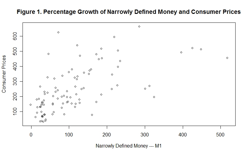
Figure 1 and Figure 2 plot the percentage rates of money and price level
increase over four ten-year periods for forty-two countries
using data obtained from the International Monetary Fund publication
International Financial Statistics. For each country,
data permitting, three sets of ratios were constructed. The growth
(end of period over beginning of period) of the Consumer Price
Indexes (CPIs) and nominal money supplies using both narrow (M1)
and broad (M2) definitions where calculated for the four
ten-year intervals, 1968-1978, 1978-1988, 1988-1998 and 1998-2008. The
comparison of M1 growth (horizontal axis) and CPI growth (vertical
axis) is shown in Figure 1. The scatter diagram shows the CPI-M1
growth combinations extending outward along a ray from the origin
along which CPI growth is slightly more than proportional to M1 growth, as
would be consistent with a decline in real money balances in situations
where inflation is greater.
In ending this Lesson we examine some empirical evidence
about the effect of the money supply on the price level and the
effects of expected inflation on real money holdings. We would
expect to observe two things---first, that major inflations were
associated with major increases in the countries' nominal money
supplies, and second, that high inflation rates tended to result
in high expected inflation rates, leading people to economize on
their real money holdings because, as we have learned, inflation
is a tax on money.
There is a clear positive association between the two variables. A comparable scatter plot using CPI and M2 growth is presented in Figure 2. The evidence clearly suggests a strong association between M2 growth and CPI growth.
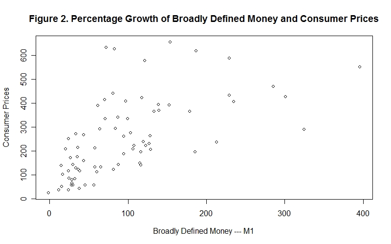
Indeed the inflation-money-growth combinations for some periods for some countries had to be eliminated from the scatter plot because the magnitudes of inflation and money growth were so large that they would dominate the plot---the scale would be such that the inflation-money-growth combinations for most of the other countries and periods would appear as a small dark mass of overlapping data points in the bottom left corner of the figure. And many countries had to be excluded from the sample because their inflation rates and money growth rates were so high that useful data were not recorded. The necessity for such omissions, of course, strengthens the conclusion that money growth and inflation were related---in all cases, high inflation was associated with high money growth. Also, no country was included for which data points for less than two periods were available.
In the case of both monetary aggregates, only loose relationships between growth of the money aggregates and growth of the CPIs obtain. This is because the demands for real money balances changed over the ten-year periods as a result of real income growth, changes in expected inflation and changes in the technology of making transactions. As would be expected, these demand-for-money effects on the price level tend to obscure the supply-of-money effects. To properly measure the money supply effects on the price levels of these countries we would have to correct for the changes in their demands for money.
It is also useful to plot countries' money supplies and CPIs in time-series form. This is done for Mexico, a high inflation country, in Figure 3. The series are indexed to 1990 = 100 but, because the growth of money and prices has been so enormous, it is necessary to use a logarithmic scale on the vertical axis. The money supply and CPI series correspond rather closely.
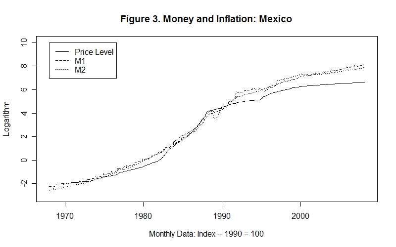
Figure 4 presents a time-series plot of the logarithms two monetary aggregates and the CPI, also indexed to 1990 = 100, for the United States, a low-inflation country. The differences in money growth and inflation between the two countries can be seen by simply comparing Figure 4 with Figure 3 and noting that the scales on their vertical axes are the same.
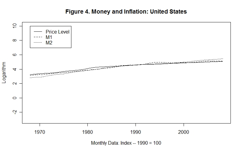
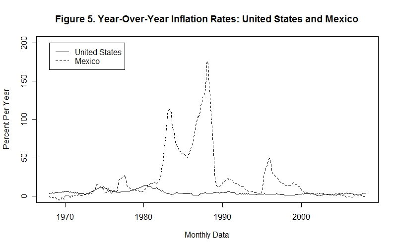
Figure 5 compares the year-over-year inflation rates of Mexico and the United States. The period of high inflation in the U.S. in the late 1970s, which prompted a change in the way monetary policy was conducted, pales to insignificance in comparison to the Mexican inflation rates ranging between 70 and 130 percent per year during the 1980s. Notice that the Mexican Government managed to get the country's inflation rate under some degree of control in the early 1990s, only to have a reoccurrence of somewhat higher inflation after the exchange rate crisis that occurred in late 1994.
The Mexican inflation rate and Mexicans' real M1 holdings are plotted in Figure 6. The money supply series is indexed to 1990 = 100. Notice how the level of real money holdings declined during the period of very high inflation in the mid-1980s and then rose back to its earlier level in the 1990s when more moderate inflation resumed. Real money holdings then fell again when the inflation rate increased in 1995 and then maintained that relatively lower level thereafter.
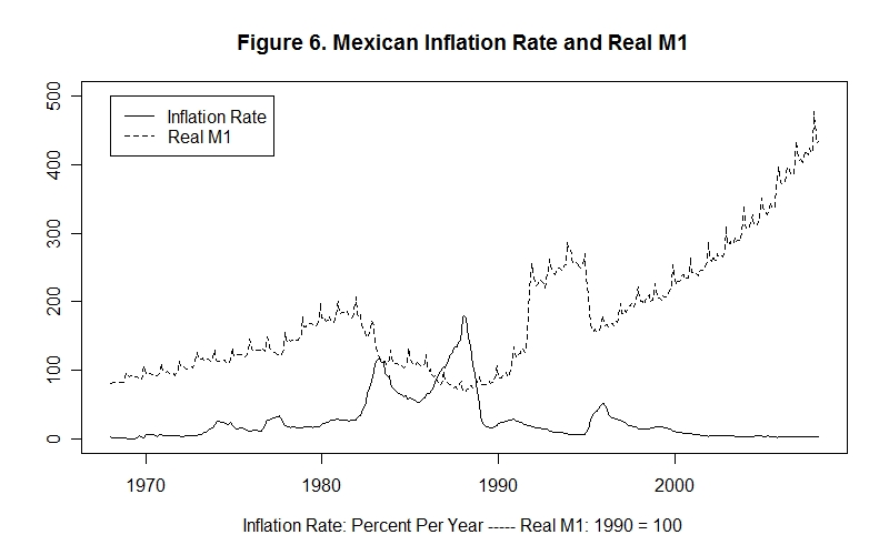
This is what we would expect. When the inflation rate rises the public's expected rate of inflation also increases. This expected higher inflation rate increases the cost of holding money as compared to other assets, causing people to reduce their real money holdings. When the inflation rate returns to its old level, expected inflation declines. The cost of holding money thus declines and the quantity of real money balances held increases. Even the relatively small increase in the inflation rate in 1995 had an effect on real money holdings---the public may have viewed the 1994 crises and resulting increase in the inflation rate as a harbinger of things to come.
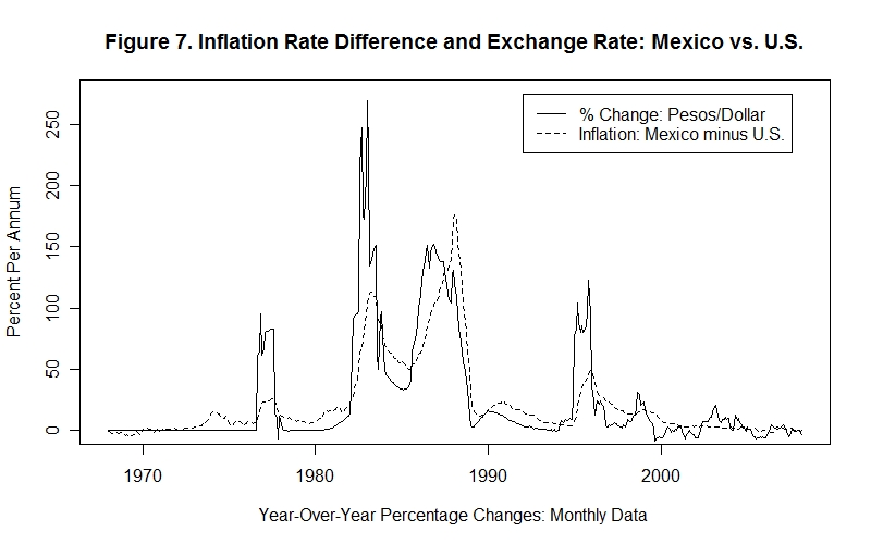
It is also interesting to look at the movements in Mexico's exchange rate with respect to the U.S. dollar. The year-to-year percentage change in the peso price of the U.S. dollar is plotted in Figure 7 along with the excess of the Mexican inflation rate over the U.S. inflation rate. The correspondence between the two series is clear. When the Mexican inflation rate was high relative to the U.S. inflation rate the rate of devaluation of the peso in terms of the U.S. dollar increased. This again is what we would expect. A decline in the internal value of the peso (that is, a fall in the amount of Mexican goods it will buy) will be accompanied by a similar decline in the peso's external value (that is, in the amount of foreign---in this case U.S.--goods it will buy).
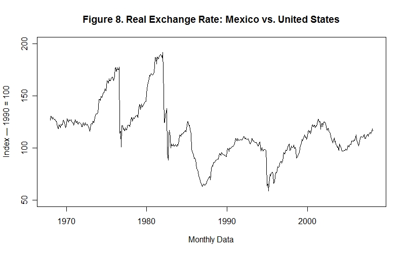
You will notice that the difference between the Mexican and U.S. inflation rates does not exactly match the rate of devaluation of the peso. This means that Mexico's real exchange rate with respect to the U.S.---that is, the relative price of Mexican goods in terms of U.S. goods measured in a single currency---was not constant during the period. The real exchange rate of Mexico vs. the U.S. is plotted in Figure 8. Variation in the real exchange rate is also to be expected. The effects of technological change and differential real investment in Mexico relative to the U.S. would be expected to cause the relative price of Mexican goods in terms of U.S. goods to change as the two economies grow.
It is time for the last test in this Lesson. As always, do yourself a favour by thinking up your own answers to the questions before looking at the ones provided.
Choose Another Topic in the Lesson