When there are only two firms in the industry, it is in their advantage
to collude and set the price and their individual outputs at levels that
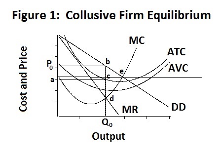
will maximize their joint profits. This situation is shown in Figure 1
where the demand curve, given by DD, is the individual firm's share of
the market demand under circumstances where the two firms are identical
with respect to size and costs of production.
We now turn to the situation when there are a small number of firms
in the industry and these firms have the option of colluding with
or competing with each other. To begin with, we assume that there are
only two firms---a situation called duopoly. Then in the next Topic
we will consider a larger number of firms---first four and then ten.
The results, as should be clear from the discussion in the previous Topic, are that each firm is a monopoly supplier of half the industry output and, given agreement that the price charged should be P{0} , chooses the output that creates equality between its marginal revenue (and the industry marginal revenue) with its own marginal costs, at point d in the Figure. It earns a profit equal to the area P0 b c a . The curves in all the Figures presented in this topic are calculated precisely using the free statistical program R and the magnitudes of the prices, quantities and profits are presented in the output file cournot.Rou. These numbers are calculated using the input file cournot.R, the contents of which also appear in the output file. Under their optimal collusive arrangement, each firm produces 435 thousand units and sells them at the collusively decided price of $41.72, earning 5187.85 thousand dollars profit. These calculations are performed under the assumption that the industry demand curve is
1. P = 70 − 0.0325 Q .
Under complete collusion, with the firms of equal size so that Q = 2 q , each individual firm's demand curve is
2. P = 70 − 0.065 q .
The marginal revenue curve of the two firms combined is obtained by calculating the change in the total revenue of the industry for each successive one-unit change in industry output---that is,
which simplifies to
3. MR = 70 − 0.065 Q
where MR is the marginal revenue of the industry. The above equation turns out to be identical to the demand curves of the individual firms. The individual firms' marginal revenue relations, assuming that both produce the same output so that Q = 2 q , is given by
4. MR = 70 − 0.13 q .
The individual firms' total, average and marginal cost curves are calculated in a fashion that makes the average cost curves U-shaped and the marginal cost curves upward sloping beyond some appropriate output level as shown in the Figures here presented.
There are two problems with collusion. First, it is illegal in most advanced industrial countries, so that any collusive arrangements can not be written down and legally enforced. Second, given this illegality, any collusive arrangement can be be profitably broken by one of the parties to the detriment of the other. Suppose that one of our two firms decides to break their collusive arrangement and to act independently, while the other firm chooses to follow that arrangement. The situation with respect to the deviant firm is presented in Figure 2 below.
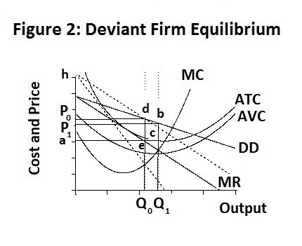
The demand for the deviant firm's output is much more elastic than the industry demand, given the constant output of the other firm, and the deviant firm's marginal revenue, denoted by MR , is also much flatter and closer to the firm's demand curve when it increases its output beyond that agreed to in the collusive arrangement. The collusive demand and marginal revenue curves are given by the dotted lines in the figure extending downward to the right from point h . The deviant firm's demand curve must pass through the collusive demand curve at the collusive price and quantity equilibrium. When the deviant firm increases its output by dq , with the other firm holding its output at the collusive level, the market price falls by the amount 0.0325 dq as can be seen from Equation 1 with dQ = dq . As shown in cournot.Rou, to equate its marginal cost with its non-collusive marginal revenue curve, the firm increases its output to 518 thousand units, lowering the market price of the good to $39.03 and increasing its profit to 5643.54 thousand dollars. Its collusive partner, whose output is assumed to remain unchanged, suffers a reduction in its profits from the previous monopoly level of 5187.85 thousand dollars to 4014.43 thousand dollars. The deviant firm increases its profits by 455.69 thousand dollars while the other firm loses 1173.42 thousand dollars, with a net loss to the two firms combined of 717.73 thousand dollars.
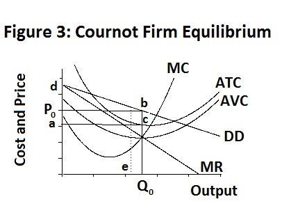
At this point, it becomes reasonable for the colluding partner firm to also break with the collusive arrangement and produce its most profitable output, given the output of its break-away partner. At that point, the break-away partner can increase its profits by adjusting its output to the most profitable level given the new level of output of the other firm. The two firms will continue to adjust their outputs in this fashion until neither firm can gain by further adjusting its output. The resulting equilibrium is called the Cournot equilibrium, after Antoine Augustin Cournot (1801-1877), and is presented in Figure 3 below which, given our assumption that the two firms are identical, represents the equilibrium of each of them.
To obtain this equilibrium we assume that each firm adjusts its output to maximize its profits, which are equal to
5. π = P(Q) q − C(q) ,
where π is the individual firm's profit, Q is the level of industry output, q is the level of output of the individual firm (where the two firms are assumed to be identical), P is the price of that output, P(Q) is the function presented in Equation 1, giving the level of P associated with each level of Q, and C(q) is a function giving the firm's total costs associated with each level of its output. To maximize its profit, each firm adjusts q until π is at its maximum, at which point
6. dπ/dq = P(Q) + q dP(Q)/dq − dC(q)/dq = P(Q) + q dP(Q)/dQ dQ/dq − dC(q)/dq = 0
which, upon rearrangement, becomes
7. P(Q) + q dP(Q)/dQ dQ/dq = dC(q)/dq .
The term dC(q)/dq is simply the marginal cost calculated in cournot.R and denoted as MC in the three Figures above. The term to the left of the equality in Equation 3 is the firm's marginal revenue, denoted below as MR, which reduces to
and becomes
8. MR = 70 − 0.0975 q
Essentially, each firm's demand curve has the same slope as in Figure 2, with its intersection with the vertical asis being lower than the intersection of the industry demand curve by an amount equal to slope of the firm demand curve multiplied by the other firm's output, under the assumption that the other firm is pricing the same way as it is. The difference between this Cournot equilibrium and the collusive one is that each firm adjusts its output independently of the other firm's output to maximize its profit, whereas under collusion it adjusts its output in conjunction with an agreed-upon equivalent adjustment of the other firm's output.
Under this equilibrium, both firms produce outputs of 506 thousand units, selling them at a price of $37.11 and earning profits of 4474.58 thousand dollars. This is 1168.96 thousand dollars less that either firm could earn if it were the only one to break the collusive arrangement and 713.27 thousand dollars less than they could each earn under complete collusion.
Of course, we can not take very seriously the magnitudes of the numbers in the example above. That example is based solely on the assumptions that the average total cost curve is U-shaped, that the industry demand curve is negatively sloped, and that the two firms are identical. These assumptions are consistent with a wide variety of possible numerical results---all that is important is the direction of the effects that arise from one or both firms breaking the collusive arrangement.
An important tool used to analyse the interaction of firms under conditions where collusion is possible but such arrangements can be easily broken is game theory analysis. The classic example for the duopoly analysis here is the prisoner's-dilemma game which can be described as follows. Suppose that there are two criminals jointly guilty of a serious crime who have been arrested by the police and are being interviewed separately and simultaneously. Each prisoner has the option of either confessing or not confessing to the crime. If neither confess a conviction will be hard to obtain and both will be convicted of a smaller crime and have to serve 1 year in jail. If one prisoner confesses but the other does not, the one who confesses will go free while the other will serve 20 years in prison. If both confess, they will each have to serve 10 years in prison. The situation is outlined in the Table below:
| Prisoner #2 | |||
| Confess | Do Not | ||
| Prisoner #1 | Confess | (-10 , -10) | (0 , -20) |
| Do Not | (-20 , 0) | (-1 , -1) | |
The numbers in brackets give the cost to Prisoner #1 on the left and the cost to Prisoner #2 on the right.
Consider the situation from the point of Prisoner #1. If he assumes that Prisoner #2 will confess, he spends 10 years in jail if he also confesses and 20 years in jail if he does not confess. If, on the other hand, he assumes that Prisoner #2 will not confess, he spends no time in jail if he confesses and 1 year in jail if he does not confess. He is better off confessing, regardless of which decision Prisoner #2 makes. The situation is exactly the same for Prisoner #2. By confessing, he serves 10 years in jail as opposed to 20 years if Prisoner #1 confesses and zero time in jail as opposed to to 1 year if Prisoner #1 does not confess. Both prisoners will thus choose to confess---neither will later wish they had done the opposite after observing what the other prisoner has decided to do. This is called a Nash equilibrium after the the famous game theorist John Nash (1929, ). Each participant adopts the strategy that is best for him regardless of which strategy the other participant chooses. Of course, in many games there is no such strategy possible, in which case a Nash equilibrium cannot occur.
Now consider the two firms in the duopoly case analyzed above. As can be seen in the Table below, the results are exactly comparable to the prisoner's dilemma game except that the Nash equilibrium is for both firms to not abide by any collusive agreement.
| Firm #2 | |||
| Collude | Do Not | ||
| Firm #1 | Collude | (5187.85 , 5187.85) | (4014.43 , 5643.54) |
| Do Not | (5643.54 , 4014.43) | (4474.58 , 4474.58) | |
Firm #1 will be better off by not colluding both in the case where Firm #2 abides by the collusive agreement and in the case where it does not, earning 5643.54 thousand dollars verses 5187.85 thousand dollars in the former case and 4474.57 verses 4014.43 in the latter case. The situation is exactly the same for Firm #2. If Firm #1 adheres to a collusive agreement Firm #2 will earn 5643.54 thousand dollars by breaking the agreement verses 5187.85 by also colluding. And if Firm #1 breaks the collusive agreement, firm #2 will earn 4474.58 thousand dollars as opposed to 4014.43 thousand dollars by also breaking it. As noted above, this equilibrium was established by Cournot, using what became a Nash equilibrium as a result of Nash's game-theory work many years later.
The question arises as to the socially efficient levels of output that the two firms should produce and the price at which that output should be sold. One way of thinking about this is to imagine the price that a government regulator should impose on the two firms to be them to produce the most efficient level of output. This can be seen with reference to Figure 4 below.
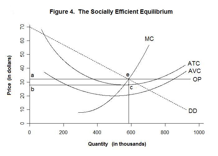
First note that the marginal cost to the firm represents the social marginal cost to the extent that it incorporates all the social costs of producing the product---that is, there are no production externalities. And the firm' demand curve, which maps the price charged against one-half of the aggregate output of the industry and is given by the dotted line DD in the Figure, gives the amount that the public is willing to pay (assuming no consumption externalities) for additional units of output as they are received. Keep in mind that this amount equals the value of other goods the public is willing to give up in order to obtain the last unit of the good consumed. So the DD curve is the marginal social return. Equating marginal social cost with marginal social return leads to the optimum output at point e in the Figure at the government imposed price of OP. That price, which in the model we numerically calculate equals $32.105, exceeds the firm's average total cost, which equals $28.003, resulting in excess profits of 2390.986 thousand dollars.Why should a properly regulated industry earn excess profits? This occurs because there is only room for two firms in the industry and the optimum output of that industry happens to be one for which the average total cost is less than the market price. If a third firm were to enter, it and the two original firms would all suffer losses. Of course, the government, after observing these profits, could impose lump-sum taxes on the firms of this magnitude---the public would receive the benefits and the firms would still find it worthwhile to continue producing the socially efficient output.
The simple example produced here vastly under-rates the problem faced by a government agency whose function is to regulate a duopoly, or even a monopoly, by imposing on it the socially efficient price. To do this, the authorities have to be able to estimate the marginal costs of the firms and the industry along with consumers' demand curve for the product. To obtain useful information about costs, they most surely have to examine evidence obtained directly from the firms, which have an obvious incentive to misrepresent their situation. Moreover, any equilibrium price, be it the monopoly price, the Cournot equilibrium price or the socially efficient price, will tend to vary through time with economic conditions---failure of the authorities to recognize the correct level and path of prices and adjust the regulated prices accordingly may result in a greater waste of resources through regulation than would be lost if the Cournot equilibrium, or even a collusive monopoly equilibrium, were allowed to rule.
In the simple example above, it would seem reasonable for the two firms to find a way to collude even when such collusion is illegal and unenforceable in the courts. All it would take is a phone call followed by a movement of the initiating firm to the collusive equilibrium. The other firm will face an obvious gain in long-run profits by also adopting that equilibrium, knowing that if it does not follow suit the initiating firm will go back to the Cournot equilibrium. The practical problem, of course, is that the range of products and services provided by such firms in the real world are not identical and demand and costs are changing through time, with new profit opportunities appearing on occasion and some current activities occasionally becoming less profitable and needing to be abandoned. Thus, even in a situation of Cournot equilibrium the firms' prices will be constantly adjusting through time and in relation to each other. To maximize its profits under Cournot equilibrium the individual firm has to make the correct pricing and production decisions, given the assumption that the other firm will also do the same. Even if the firms have informally agreed to collude, one of them can always argue that its recent reduction in the price of its output or, say, the free provision of associated services, was the result of factors specific to its situation and not a violation of the collusive agreement, even though it may in fact be deliberately violating that agreement. So the best understanding we can arrive at is that the prices charged by the duopolists are likely to be at the Cournot equilibrium level or somewhere above, yet probably below the level possible with complete collusion.
One way in which the two firms above could maximize their value is to merge into a single firm, either by one firm purchasing the other or by both firms selling out to a third party who would be willing to pay them more than the present value of future Cournot-equilibrium profits in order to create a single monopoly firm. The problem is that these actions would probably encounter legal prohibition or subsequent government regulation in most advanced industrial countries.
It is now time for a test. For your own intellectual enlightenment, think up complete answers to the questions before looking at the ones provided.
Choose Another Topic in the Lesson